Post last updated 11 May 2018. See end of post for details.
While journeys to work only represents around a quarter of all trips in Melbourne, they represent around 39% of trips in the AM peak (source: VISTA 2012-13). Thanks to the census there is incredibly detailed data available about the journey to work, and who doesn’t like exploring transport data in detail?
Between 2006 and 2016, Melbourne has seen mode shifts away from private transport and walking, and towards public transport and cycling. The following measures are by place of enumeration (and 2011 Significant urban area boundaries):
| 2006 | 2011 | 2016 | |
| Public transport (any) | 14.16% | 16.34% | 18.15% |
| +2.18% | +1.82% | ||
| Private transport (only) | 80.43% | 78.16% | 76.20% |
| -2.28% | -1.96% | ||
| Walk only | 3.63% | 3.46% | 3.47% |
| -0.18% | +0.01% | ||
| Bicycle only | 1.34% | 1.56% | 1.63% |
| +0.23% | +0.06% |
This post unpacks where mode shifts and trip growth is happening, by home locations, work locations, and home-work pairs. It tries to summarise the spatial distribution of journeys to work in Melbourne. It will also look at the relationship between car parking, job density and mode shares.
I’m afraid this isn’t a short post. So get comfortable, there is much fascinating data to explore about commuting in Melbourne.
Public transport share by home location
Here’s an animated public transport mode share map 2006 to 2016 – you might want to click to enlarge, or view this map in Tableau (be patient it can take some time to load and refresh). For those with some colour-blindness, you can also get colour-blind friendly colour scales in Tableau.
![]()
The higher mode shares pretty clearly follow the train lines and the areas covered by trams, with mode share growing around these lines. Public transport mode shares of over 50% can be found in a sizeable patch of Footscray, and pockets of West Footscray, Glenroy, Ormond – Glen Huntly, Murrumbeena, Flemington, Docklands, Carlton, and South Yarra. Larger urban areas with very low public transport mode share can be found around the outer east and south-east of the city, particularly those remote from the rail network.
Here’s a map showing mode shift at SA2 level:
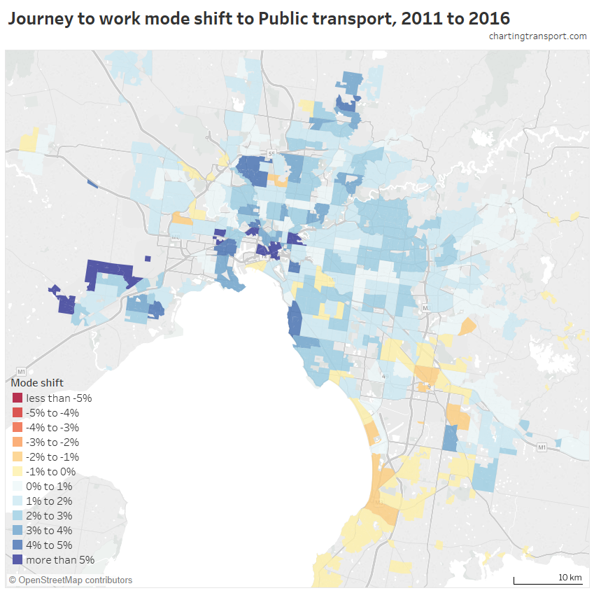
(explore in Tableau)
The biggest shifts to public transport in the middle and outer suburbs were in Wyndham Vale, Tarneit, South Morang, Lynbrook/Lyndhurst, Sanctuary Lakes (Point Cook – East), Truganina / Williams Landing, Rockbank, Pascoe Vale, and Glenroy. That’s almost a roll call of all the new train stations opened between 2011 and 2016. The exceptions are Rockbank (a small community at present which received significantly more frequent trains in 2015), Point Cook East (a bus service was introduced in 2015), and Pascoe Vale / Glenroy (where more people are commuting to the city centre and increasingly by public transport).
Inner suburban areas with high mode shifts include West Footscray, Yarraville, Seddon – Kingsville, Collingwood, Abbotsford, Kensington, Flemington, South Yarra – East, and Brighton. The Melbourne CBD itself had a 13% shift to public transport – and actually a 6% mode shift away from walking (which probably reflects the new Free Tram Zone in the CBD area).
The biggest mode shifts away from public transport (of 1 to 2%) were at Ardeer – Albion, Coburg North, Chelsea – Bonbeach, Seaford, Frankston, Dandenong, Hampton Park – Lynbrook, and Lysterfield. At the 2016 census there were no express trains operating on the Frankston railway line due to level crossing removal works, which might have slightly impacted public transport demand in Frankston, Seaford and Chelsea – Bonbeach. I’m not sure of explanations for the others, but these were not large mode shifts.
Here’s a chart showing mode split over time, by home distance from the CBD:
Public transport mode share by work location
Here’s a map showing work location public transport mode share (Destination Zones with less than 5 travellers per hectare not shown):
![]()
It’s no surprise that public transport mode share is highest in the CBD and surrounding area, and lower in the suburbs. But note the scale – public transport mode share falls away extremely quickly as you move away from the city centre.
Private transport mode shares are very high in the middle and outer suburbs:
![]()
Large areas of Melbourne have near saturation private transport mode share. In most suburban areas employee parking is likely to be free and public transport would struggle to compete with car travel times, even on congested roads (particularly for buses that are also on those congested roads).
There are some isolated pockets of relatively high public transport mode share in the suburbs, including
- 34% in a pocket of Caulfield – North (right next to Caulfield Station),
- 33% in a pocket of Footscray (includes the site of the new State Trustees office tower near the station),
- 25% in a pocket of Box Hill near the station, and
- 17% at the Monash University Clayton campus.
Explore the data yourself in Tableau.
Here’s an enlargement of the inner city area:
![]()
And here’s a map showing the mode shift between 2011 and 2016 by workplace location (for SA2s with at least 4 jobs per hectare):
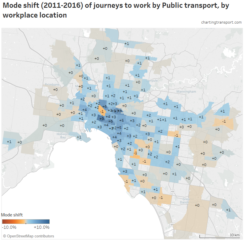
The biggest shifts to public transport were in the inner city. The biggest shifts away from public transport were 1.4% in Ormond – Glen Huntly (rail stations temporarily closed) and North Melbourne.
Here’s a closer look at the inner city:
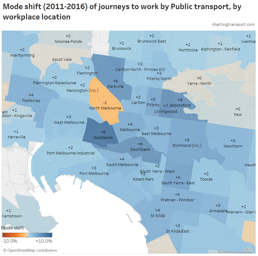
Docklands had the highest mode shift to public transport of 9% (almost all of it involving train) followed by Collingwood with 7%, and Parkville, Southbank, and Abbotsford with 6%.
North Melbourne saw a decline of 1.4% – at the same time private transport mode share and active (only) mode shares increased by 1%.
Another way to slice this data is by distance from the CBD. Here are main mode shares by workplace distance from the centre, over time:

For this and several upcoming pieces of analysis, I have aggregated journeys into three “main mode” categories:
- Public transport (any trip involving public transport)
- Private transport (any journey involving private transport that doesn’t also involve public transport)
- Active transport only (walking or cycling)
Here are the mode shifts by workplace distance from the centre between 2006 and 2016:
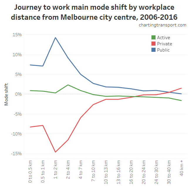
The biggest mode shift from private to public transport was for distances of 1-2km from the city centre, which includes Docklands, East Melbourne, most of Southbank, and southern Carlton and Parkville (see here for a reference map). A mode shift to public transport (on average) was seen for workplaces up to 40km from the city centre. The biggest mode shift to active transport was for jobs 2-4 km from the city centre (but do keep in mind that weather can impact active transport mode shares on census day).
What about job density?
Up until now I’ve been looking at mode shifts by geography – but the zones can have very different numbers of commuters. What matters more is the overall change in volumes for different modes. A big mode shift for a small number of journeys can be a smaller trip count than a small mode shift on a large number of journeys.
Firstly, here’s a map of jobs per hectare in Melbourne (well, jobs where someone travelled on census day and stated their mode, so slight underestimates of total employment density):

Outside the city centre, relatively high job density destination zones include:
- Heidelberg (Austin/Mercy hospitals with 10.2% PT mode share),
- Monash Medical Centre in Clayton (8.3% PT mode share),
- Northern Hospital (3.8% PT mode share),
- Victoria University Footscray Park campus (21.1% PT mode share),
- Swinburne University Hawthorn (39.8% PT mode share),
- a pocket of Box Hill (19.9% PT mode share),
- a zone including the Coles head office in Tooronga (11.2% PT mode share),
- an area near Camberwell station (26.8% PT mode share),
- a pocket of Richmond on Church Street (27.8% PT mode share), and
- a pocket of Richmond containing the Epworth Hospital (39.5% PT mode share).
Explore this map in Tableau.
You’ll probably not be very surprised to see that there is a very strong negative correlation between job density and private transport mode share. The following chart shows the relationship between the two for each Melbourne SA2 with the thin end of each “worm” being 2006 and the thick end 2016 (note: the job density scale is exponential):
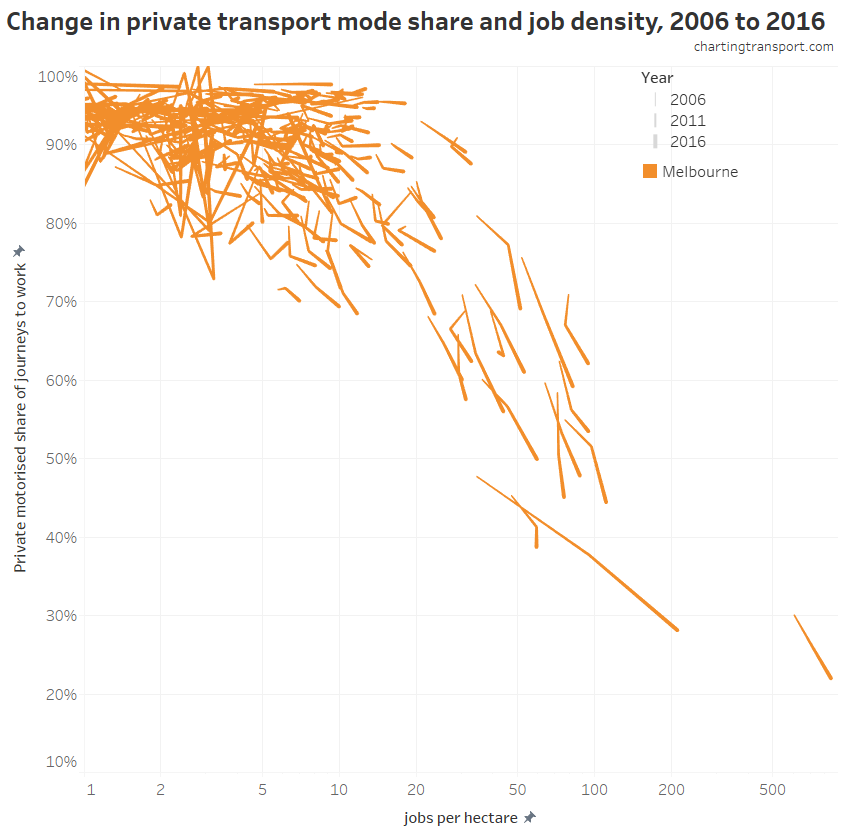
Correlation of course is not necessarily causation – high job density doesn’t automatically trigger improved public and active transport options. But parking is likely to be more expensive and/or less plentiful in areas with high employment density, and many employers will be attracted to locations with good public transport access so they can tap into larger labour pools.
The Melbourne CBD SA2 is at the bottom right corner of the chart, if you were wondering.
The Port Melbourne Industrial and Clayton SA2s are relatively high density employment areas with around 90% private transport mode shares.
Here’s a zoom in on the “middle” of the above chart, with added colour and labels to help distinguish the lines:
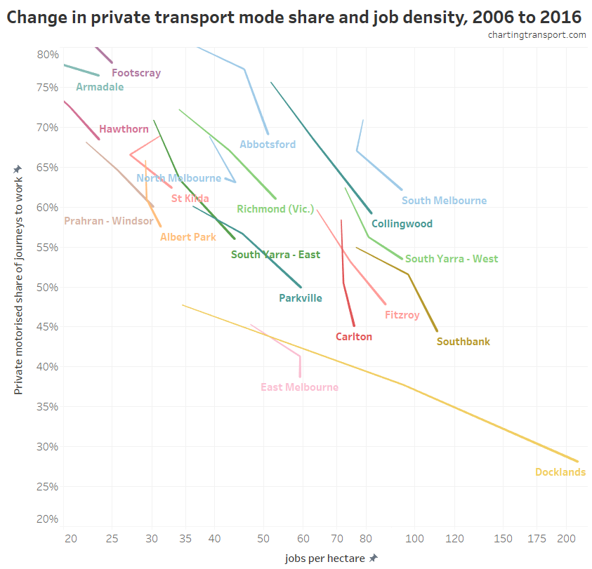
Not only is there a strong (negative) relationship between job density and private transport mode share, most of these SA2s are moving down and to the right on the chart (with the exception of North Melbourne which saw only small change between 2011 and 2016). However the correlation probably reflects many new jobs being created in areas with good public and active transport access, particularly as Melbourne grows its knowledge economy and employers want access to a wide labour market.
How does private transport mode share relate to car parking provision?
Do more people drive to work if parking is more plentiful where they work?
Thanks to the City of Melbourne’s Census of Land Use and Employment, I can create a chart showing the number of non-residential off-street car parks per 100 employees in the City of Melbourne (which I will refer to as “parking provision” as shorthand):
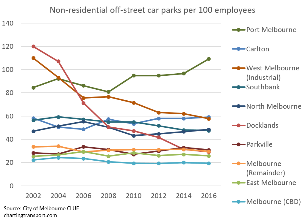
(see a map of CLUE areas)
Car parking provision per employee has increased in Carlton, North Melbourne and Port Melbourne and decreased in Docklands, West Melbourne (industrial), and Southbank. Docklands had the highest car parking provision in 2002 but this has fallen dramatically and land has been developed for employment usage. Southbank, which borders the CBD, has relatively high car park provisioning – much higher than Docklands and East Melbourne.
Here’s the relationship between parking provision and journey to work private transport mode share between 2006 and 2016:

It’s little surprise to see a strong relationship between the two, although Carlton is seeing increasing parking provision but decreasing private transport mode share (maybe those car parks aren’t priced for commuters?).
If all non-resident off street car parks were used by commuters, then you would expect the private transport mode share to be the same as the car parks per employee ratio.
Private transport mode shares were much the same as parking provision rates in Melbourne CBD, Docklands, and Southbank, suggesting most non-residential car parks are being used by commuters (with the market finding the right price to fill the car parks?). Private transport mode share was higher than car parking provision in East Melbourne, Parkville, South Yarra, North Melbourne, and West Melbourne (industrial). This might be to do with on-street parking and/or more re-use of car parks by shift workers (eg hospital workers).
Port Melbourne parking provision is very high (there is also lots of on-street parking). It’s possible some people park in Port Melbourne and walk across Lorimer Street (the CLUE border) to work in “Docklands” (which includes a significant area just north of Lorimer Street). It’s also likely that many parking spaces are reserved for visitors to businesses. Carlton similarly had higher parking provision than private transport mode share (again, could be priced for visitors).
(Data notes: For 2011, I have taken the average of 2010 and 2012 data as CLUE is conducted every even year. I’ve done a best fit of destinations zones to CLUE areas, which is not always a perfect match)
Where are the new jobs and how did people get to them?
Here’s a map showing the relative number of new jobs per workplace SA2, and the main mode used to reach them:
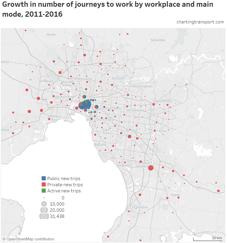
The biggest growth in jobs was in the CBD (+31,438), followed by Docklands (+22,993), Dandenong (+11,136), and then Richmond (+6,242).
And here’s an enlargement of the inner city:
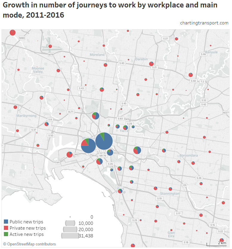
(explore this data in Tableau)
The CBD added 31,438 jobs, and almost all of those were accounted for by public transport journeys, although 2,630 were by active transport, and only 449 new jobs by private transport (1%).
Likewise most of the growth in Docklands and Southbank was by public transport, and then in several inner suburbs private transport was a minority a new trips.
However, Southbank still has a relatively high private transport mode share of 46% for an area so close to the CBD. The earlier car parking chart showed that Southbank has about one off-street non-residential car park for every two employees. These include over 5000 car parks at the Crown complex alone (with $16 all day commuter parking available as at November 2017). It stands to reason that the high car parking provision could significantly contribute to the relatively high private transport mode share, which is in turn generating large volumes of radial car traffic to the city centre on congested roads. Planning authorities might want to consider this when reviewing applications for new non-residential car parks in Southbank.
Here’s a chart look looking at commuter volumes changes by workplace distance from the CBD (see here for a map of the bands).
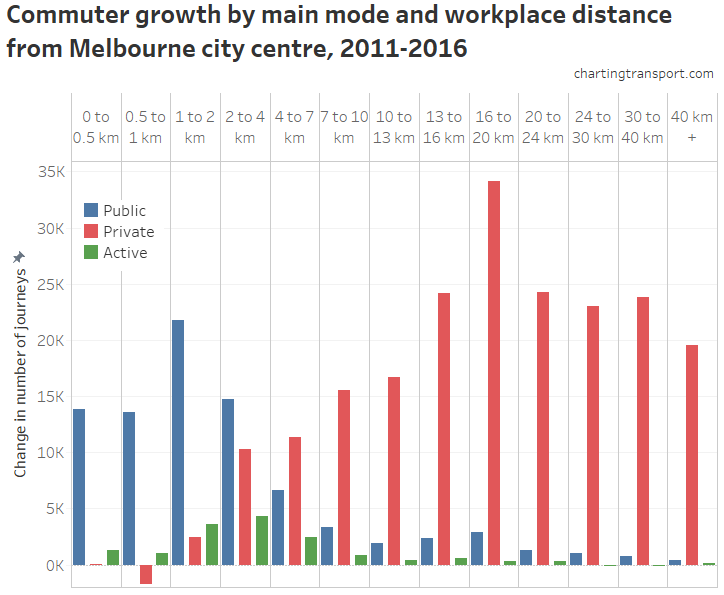
(Note: the X-axis is quasi-exponential)
Public transport dominated new journeys to work up to 4km from the city centre. Private transport dominated new journeys to workplaces more than 4km from the city centre – however that doesn’t necessarily mean a mode shift away from public transport if the new trips have a higher public transport mode share than the 2011 trips. Indeed there was a mode shift towards public transport for workplaces in most parts of Melbourne.
Here is a map showing the private transport mode share of net new journeys to work by place of work:

Private transport had the lowest mode share of new jobs in the inner city. As seen on the map, some relative anomalies for their distance from the CBD include Box Hill (64%), Hampton (57%), Brunswick East (34%), Dingley Village (28%), and Albert Park (6%). Explore the data in Tableau.
Where did the new commuters come from and what mode did they use?
Here’s a map showing the (relative) net volume change of private transport journeys to work, by home location:
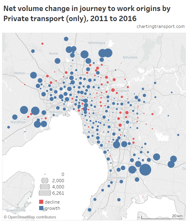
As you can see many of the new private transport journeys to work commenced in the growth areas, although there were also some substantial numbers from inner suburbs such as South Yarra, Richmond, Braybrook, Maribyrnong and Abbotsford.
There are many middle suburban SA2s with declines. These are also suburbs where there has been population decline – which I suspect are seeing empty nesting (adult children moving out) and people retiring from work. For example Templestowe generated 566 fewer private transport trips, 28 fewer active transport only trips, but only 70 new public transport trips.
Here’s a similar map showing change in public transport journeys:
![]()
The biggest increases were from the inner city, with the CBD itself generating the largest number of new public transport trips (including almost 2500 journeys involving tram). However there were a number of new public transport trips from the Wyndham area in the south-west (where new train stations opened).
Here’s a map of the total new trip volume and main mode split:
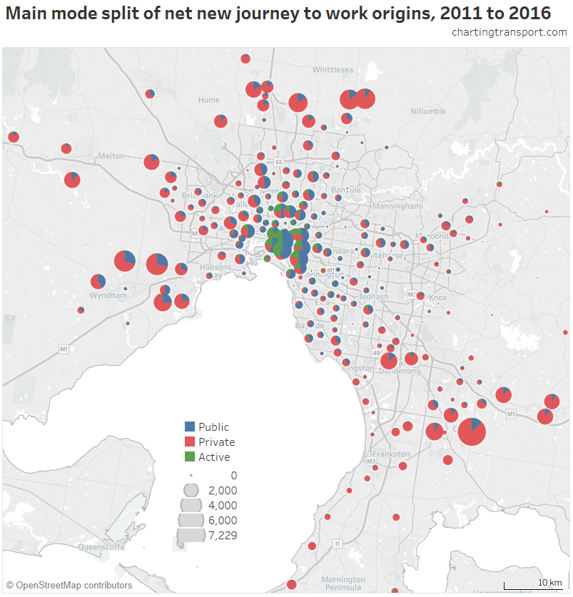
(explore in Tableau)
You can see that private transport dominates new journeys from the outer suburbs, but less so in the south-west where a new train line was opened. The middle and inner suburbs are hard to see on that map, so here is a zoomed in version:
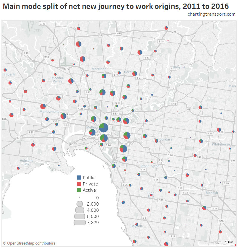
You can see many areas where private transport accounted for a minority of new trips. Also, around half of new trips in several middle northern suburbs were by public transport.
Here’s how it looks by distance from the city centre:

Public transport dominated new journeys to work for home locations up until 10km from the city centre, was roughly even with private transport from 10km to 20km (hence a net mode shift to public transport). However private transport dominated new commuter journeys beyond 20km – most of which is from urban growth areas. The 24-30 km band covers most of the western and northern growth areas, while the 40km+ band is almost entirely the south-east growth areas.
Here is a view of the private transport mode share of net new trips:

(explore in Tableau)
The pink areas had a net decline in the number of private transport trips (or total trips) generated, so calculating a mode share doesn’t make a lot of sense. There are some areas with 100%+ which means more new private transport trips were generated than total new trips – ie active and/or public transport trips declined.
You can again see that private transport dominated new trips in the most outer suburbs, with notable exceptions in the west:
- Wyndham in the south-west where two new train stations opened. 41% of new trips from Wyndham Vale and 30% of new trips from Tarneit were by public transport.
- Sunbury in the north-west, to which the Metro train network was extended in 2012. Around 37% of new trips from Sunbury -South were by public transport (that’s 307 trips).
How has the distribution of home and work locations in Melbourne changed by distance from the city?
Here’s a chart showing the number of journey to work origins and destinations by distance from the city centre by year. Note the distance intervals are not even, so look for the vertical differences in this chart:

You can see most of the worker population growth (origins) has been in the outer suburbs. The destination (job) growth was much more concentrated in the inner city between 2006 and 2011, but then more evenly distributed across the city in 2016.
The median distance of commuter home locations from the city centre increased from 18.2 km in 2006 to 18.6 km in 2016. The median distance from the city centre of commuter workplaces decreased from 13.3 km in 2006 to 12.8 km in 2011 but then increased back to 13.3 km in 2016.
Here’s another way at looking at the task. I’ve split Melbourne by SA2 distance from the CBD (to create 10km wide rings) for home and work locations (and further split out the CBD as a place of work) to create a matrix. Within each cell of the matrix is a pie chart – the size of which represents the relative number of commuter trips between that home and work ring, and the colours showing the main mode. I’ve then animated it over 2011 and 2016 (to make it five dimensional!).

I think this chart fairly neatly summarises journeys to work in Melbourne:
- Private transport dominates all journeys that stay more than 5km from the city centre (all but top left corner)
- Active transport is only significant for commuters who work and live in the same ring (diagonal top left – bottom right), or for trips entirely within 15 km of the centre (six cells in top left corner)
- Public transport dominates journeys to the CBD, no matter how far away people’s homes are, but the number of such journeys falls away rapidly with home distance from the CBD. Very few people commute from the outer suburbs to the CBD.
- Private transport commuters are mostly travelling between middle suburbs, not to the CBD or even the to within 5 km of the city. However on average they are travelling towards the centre. This will become clearer shortly.
- Public transport otherwise only gets 15% or better mode share for trips to within 5 km of the centre or the relatively small number of outward trips from the inner 5km.
Here’s a look at the absolute change in number of trips between the rings:

You can see:
- A significant growth in private transport trips, particularly within 5 – 25 km from the CBD.
- A significant growth in public transport trips, mostly to the CBD and areas within 5 km from the CBD.
Where are commuters headed on different modes?
This next analysis looks at the distribution of origins and destinations for people using particular modes, which can be compared to all journeys.
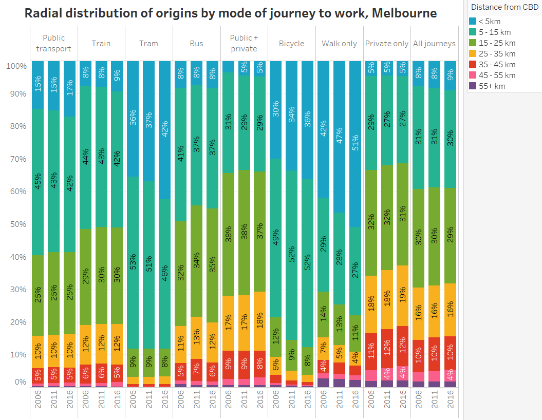
The next chart looks at the distributions of work destinations by main mode for each census year (using a higher resolution set of distances from the CBD).
On the far right is the distribution of jobs across Melbourne (with roughly equal numbers in each distance interval), and then to the left you can see the distribution of workplace locations for people who used particular modes. You can see how different modes are more prominent in different parts of the city.
You might need to click to enlarge to read the detail.

In 2016, trips to within 2km of the city centre accounted for 19% of all journeys, but 62% of public transport journeys, 31% of walking journeys, and only 7% of private transport only journeys.
Train, tram, and bicycle journeys are biased towards the inner city, while private transport only journeys are biased to the outer suburbs. Walking and bus journeys are only slightly biased towards the inner city. This should come as no surprise given the maps above showing high public transport mode shares in the inner city and very high private transport mode shares in most of the rest of the city.
Over time, public transport journeys to work became less likely to be to the central city as public transport gained more trips to the suburbs. However bus journeys to work became more likely to be in the city centre (this probably reflects the significant upgrades in bus services between the Doncaster area and city centre).
Notes on the data:
- Unless a mode is labelled “only”, then I’ve counted journeys that involved that mode (and possibly other modes).
- Sorry I don’t have public transport mode specific data for 2006 so there are some blank columns.
Where do commuters using different modes live?
Here’s the same breakdown, but by home distance from the city centre:
Private transport commuters were slightly more likely to come from the middle and outer suburbs. Tram and bicycle commuters were much more likely to come from the inner city. Bus commuters were over-represented in the 15-25 km band – probably dominated by the Doncaster area. Train commuters were over-represented in distances 5-25 km from the city, and under-represented in distances 35 km and beyond. Journeys by both public and private transport were more likely to come from the middle suburbs.
51% of people walking to work live within 5 km of the city centre, and the growth in walking journeys to work has been much stronger in the inner city.
Here’s a chart showing the most common home-work pairs for distance rings from the CBD for public transport journeys. It’s like a pie chart, but rectangular, larger and much easier to label (I haven’t labelled the small boxes in the bottom right hand corner):

You can see the most common combination is from 5-15 kms to 0-5 kms. This is followed by 15-25 to 0-5 kms and 0-5 to 0-5 kms.
Here’s the same for private transport only journeys:

There is a much more even distribution.
Finally, here is the same for active-only journeys to work:

This is much more polarised, with almost 40% of active transport trips being entirely within 5 km of the city centre. The second most common journey is within 5-15km of the city followed by from 5-15 km to 0-5 km.
In future posts I will look at more specific mode shares and shifts in more detail, the relationship between motor vehicle ownership and journey to work mode shares, and much more!
I hope you have found this analysis at least half as interesting as I have.
(note: this post uses data re-issued in December 2017 after ABS pulled the original Place of Work data in November 2017 due to quality concerns)
This post was updated on 24 March 2018 with improved maps. Also, data reported at SA2 level is now as extracted at SA2 level for 2011 and 2016, rather than an aggregation of CD/SA1/DZ data (each of which has small random adjustment for privacy reasons, which amplifies when you aggregate, also some work destinations seem to be coded to an SA2 but not a specific DZ). This does have a small impact, particularly for mode shifts and mode shares of new trips. On 7 April 2018 this post was updated to count journeys by “Other” and “Bicycle, Other” as private transport to ensure completeness of total mode share (we don’t actually know what modes “Other” is, so this isn’t perfect).
This post was further updated on 11 May 2018 to include minor adjustments to DZ workplace counts in 2011 to account for jobs where the SA2 was known but the DZ was not, and to improve mapping from 2011 DZs to 2016 SA2s. Refer to the appendix in the Brisbane post for all the details about the data.


 Posted by chrisloader