How radial is general travel in Melbourne? (part 2)

Wed 11 September, 2019

In part 1 of this series, I looked at the radialness of general travel around Melbourne based on the VISTA household travel survey. This part 2 digs deeper into radialness by time of the day and week, and maps radialness and mode share for general travel around Melbourne.

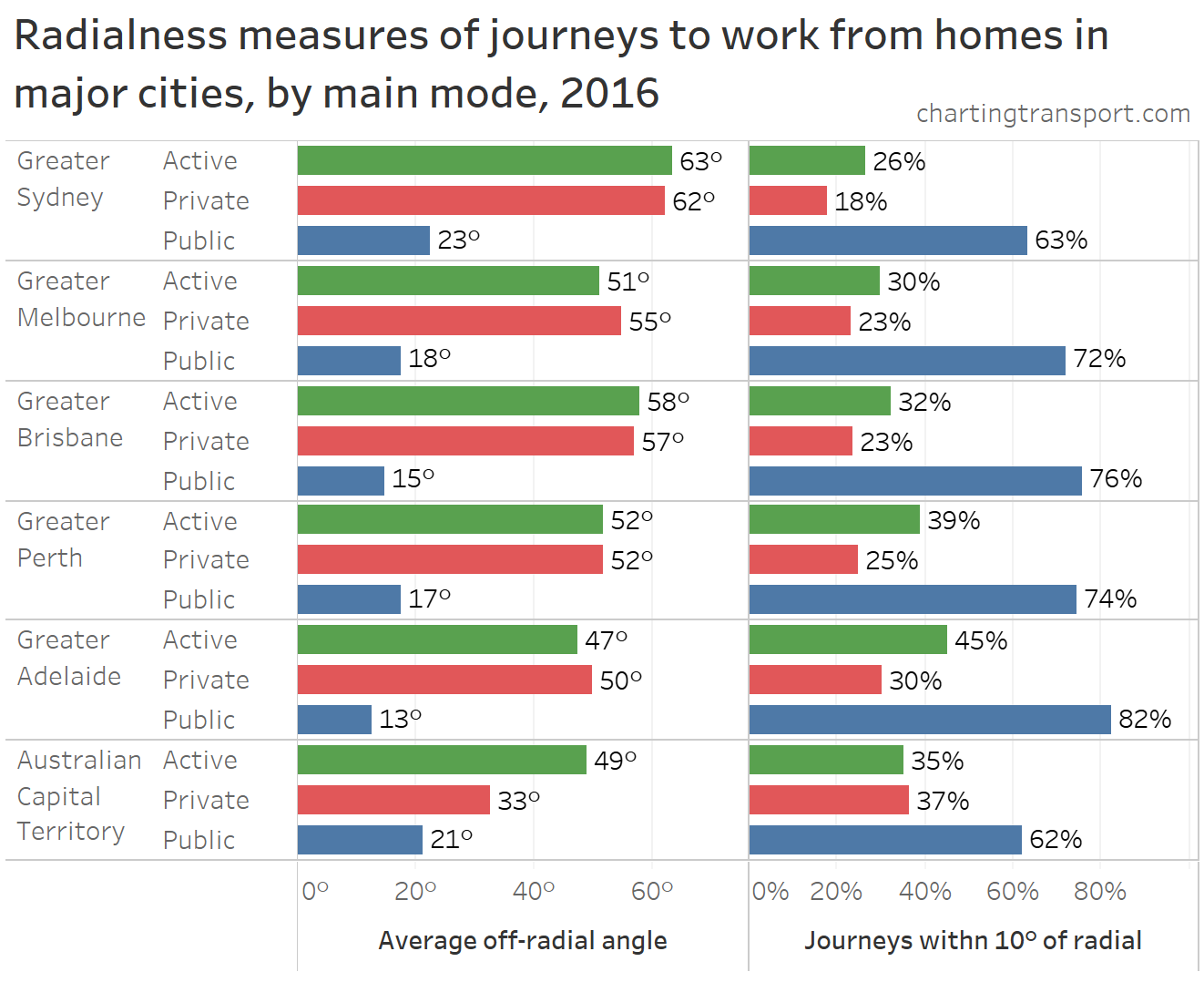
A brief recap on measuring radialness: I’ve been measuring the difference in angle between the bearing of a trip, and a straight line to the CBD from the trip endpoint that is furthest from the CBD (origin or destination). An angle of 0° means the trip is perfectly radial (directly towards or away from the CBD) while 90° means the trip is entirely orbital relative to the CBD. An average angle in the low 40s means that there isn’t really any bias towards radial travel. I’ve been calling this two-way off-radial angle. Refer to part 1 if you need more of a refresher.

How does trip radialness vary by time of week?

The first chart shows the average two-way off-radial angle for trips within Greater Melbourne by time and type of day, for private transport, public transport, and walking.

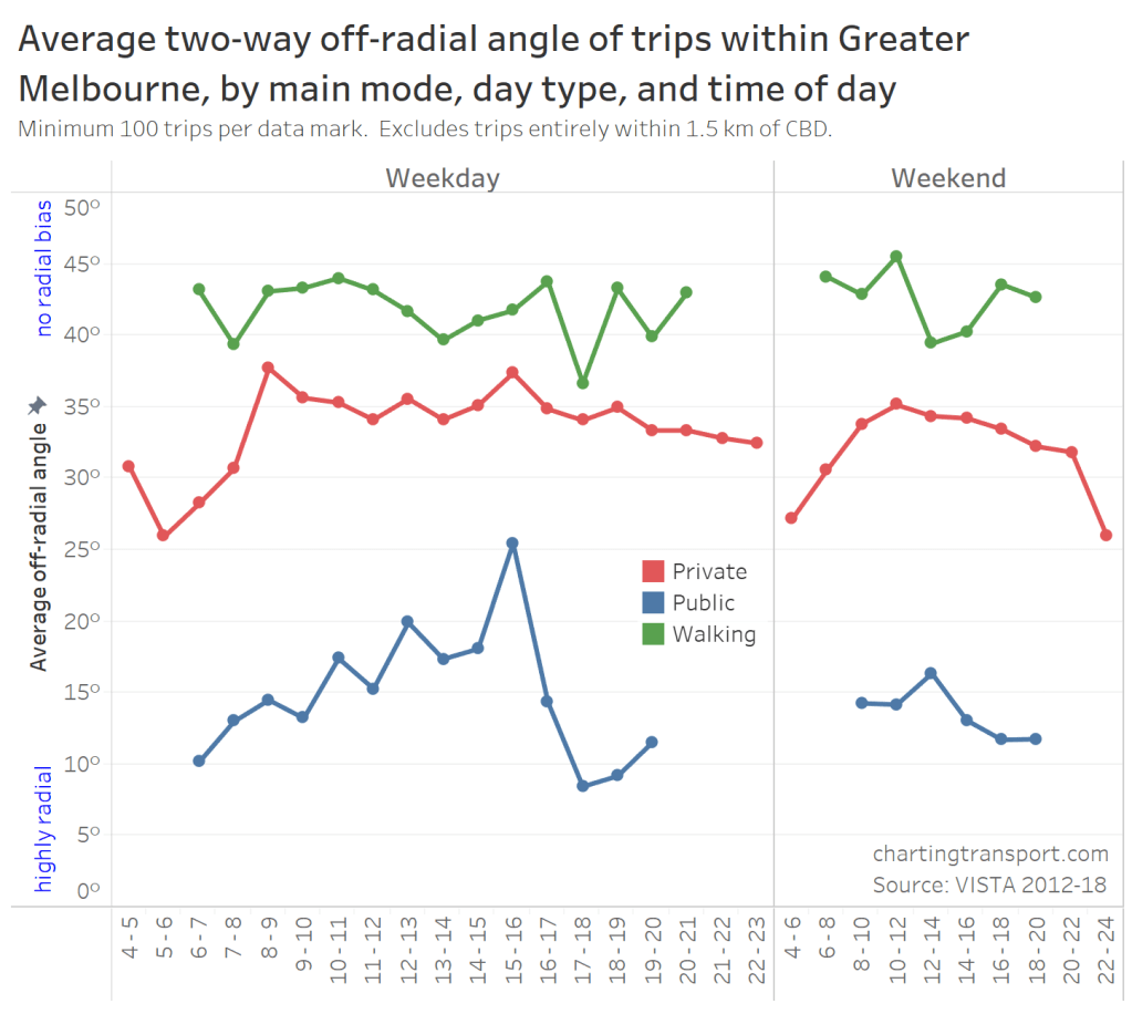
Technical notes: I’ve had to aggregate weekend data into two hour blocks to avoid issues with small sample sizes. I’m only showing data where there are at least 100 trips for a mode and time (that’s still not a huge sample size so there is some “noise”). Trips times are assigned by the clock hour of the middle of the trip duration. For example, a trip starting at 7:50 am and finishing at 9:30 am has a mid-trip time of 8:40 am and therefore is counted in 8 – 9 am for one hour intervals, and 8 – 10 am for two hour intervals.

You can see:

  • Public transport trips are much more radial at all times of the week, but most particularly in the early AM peak and in the PM commuter peak. They are least radial in the period 3-4 pm on weekdays (PM school peak), which no doubt reflects school student travel, which is generally less radial.
  • Private transport trips are more radial before 8 am on weekdays, and in the early morning and late evening on weekends. Curiously private transport trips in the PM peak don’t show up as particularly radial, possibly because there is more of a mix of commuter and other trips at that time.
  • Walking trips show very little radial bias, except perhaps in the commuter peak times on weekdays.

When I drill down into specific modes, the sample sizes get smaller, so I have used 2 hour intervals on weekdays, and 3 hour intervals on weekends. Also to note is that VISTA assigns a “link mode” to each trip, being the most important mode used in the journey (generally train is highest, followed by tram, bus, vehicle driver, vehicle passenger, bicycle, walking only). I am using this “link mode” in the following charts.

Some observations:

  • Train trips are the most radial, followed by tram trips (no surprise as these networks are highly radial).
  • Bicycle trips are generally the third most radial mode, except at school times.
  • Public bus trips are more radial in the commuter peak periods, and much less radial in the middle of the day on weekdays. The greater radialness in commuter peaks will likely reflect people using buses in non-rail corridors to travel to the city centre (particularly along the Eastern Freeway corridor). Most of Melbourne’s bus routes run across suburbs, rather than towards the city centre, which will likely explain bus-only trips being less radial than train and tram, particularly off-peak.

How does radialness vary by trip purpose and time of week?

The following chart shows the average two-way off-radial angle of trips by trip purpose (at destination) and time of day:

Some observations:

  • Work related trips are generally the most radial, particularly in the AM peak (as you might expect), but less so on weekdays afternoons.
  • Weekday education trips are the next most radial (excluding trips to go home in the afternoon and evening), except at school times (school travel being less radially biased than tertiary education travel).
  • Social trips become much more radial late at night on weekends, probably reflecting inner city destinations.
  • Recreational trips are the least radial on weekends.
  • Otherwise most other trip purposes average around 35-40° – which is only slightly weighted towards radial travel.

What is the distribution of off-radial angles by time of day?

So far my analysis has been looking at radialness, without regard to whether trips are towards or away from the CBD. I’ve also used average off-radial angles which hides the underlying distribution of trip radialness.

I’m curious as to whether modes are dominated by inbound or outbound trips at any times of the week (particularly private transport), and the distribution of trips across various off-radial angles.

So to add the inbound/outbound component of radialness, I am going to use a slightly different measure, which I call the “one-way off-radial angle”. For this I am using a scale of 0° to 180°, with 0° being directly towards the CBD, and 180° being directly away from the CBD, and 90° being a perfectly orbital trip with regard to the CBD. For inbound trips, the one-way off-radial angle will be the same as the two-way off-radial angle, but outbound trips will instead fall in the 90° to 180° range.

One-way off-radial angles are still calculated relative to the trip end point (origin or destination) that is furthest from the CBD. I explained this in part 1.

Here is the distribution of one-way off-radial angles by time of day for trips where train was the main mode:

A reminder: only time intervals with a sample of at least 100 trips are shown.

In the morning, trips are very much inbound radial, with around three-quarters being angles of 0°-10°. Likewise in the PM peak, almost three-quarters of train trips are very outbound radial with angles 170°-180°.

As per the second chart in this post, train trips remain very radial throughout the day. But there is slightly more diversity in off-radial angles 3-4 pm on weekdays, when many school students use trains for journeys home from school that are less radially biased. Less radial trips could be a result of using two train lines, using bus in combination with train, or using a short section of the train network that isn’t as radial (eg Eltham to Greensborough, Williamstown to Newport, or a section of the Alamein line).

On weekends it’s interesting to see that there are many more inbound than outbound journeys between 12 pm and 2 pm on weekends. The “flip time” when outbound journeys outnumber inbound journeys is probably around 2 pm. This is consistent with CBD pedestrian counters that show peak activity in the early afternoon.

One problem with the chart above is that volumes of train travel vary considerably across the day. So here’s the same data, but as (estimated) average daily trips:

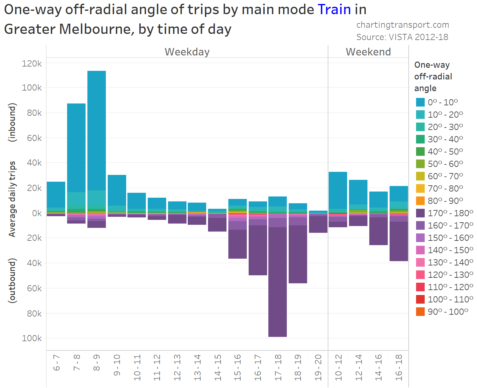
You can see the intense peak periods on weekdays, and a gradual switch from inbound trips to outbound trips around 1 pm on weekdays. There’s also a mini-peak in the “contra-peak” directions (outbound trips in the AM peak and inbound trips in the PM peak).

The weekend volumes are for two hour intervals so not directly comparable to weekdays (which are calculated for one hour intervals), but you can see higher volumes of inbound trips until around 2 pm, and then outbound trip volumes are higher.

Those results for trains were probably not surprising, but what about private vehicle driver trips?

There is much more diversity in off-radial angles at all times of the day, and a less severe change between inbound and outbound trips across the day.

On both weekday and weekend mornings there is a definite bias towards inbound travel. Afternoons and evenings are biased towards outbound travel, but not nearly as much (it’s much stronger late at night). This is consistent with the higher average two-way off-radial angle seen for private transport in the PM peak compared to the AM peak.

Here is the same data again but in volumes:

This shows the weekday AM peak spread concentrated between 8 and 9 am, while the PM peak is more spread over three hours (beginning with the end of school).

Here are the same two charts for tram trips (the survey sample is smaller, so we can only see results for weekdays):

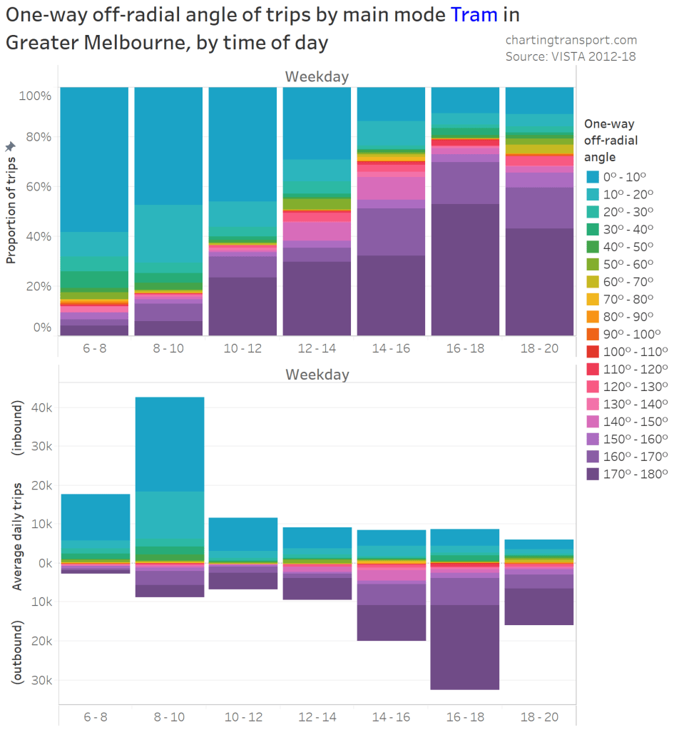
Again there is a strong bias to inbound trips in the morning and outbound in the afternoon, with slightly more diversity in the PM school peak, and early evening.

Next up public bus (a separate category to school buses, however many school students do travel on public buses):

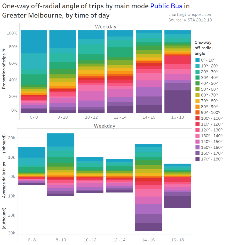
There is a lot more diversity in off-radial angles (particularly 2-4 pm covering the end of school), but also the same trend of more inbound trips in the morning and outbound trips in the afternoon.

Next up, bicycle:

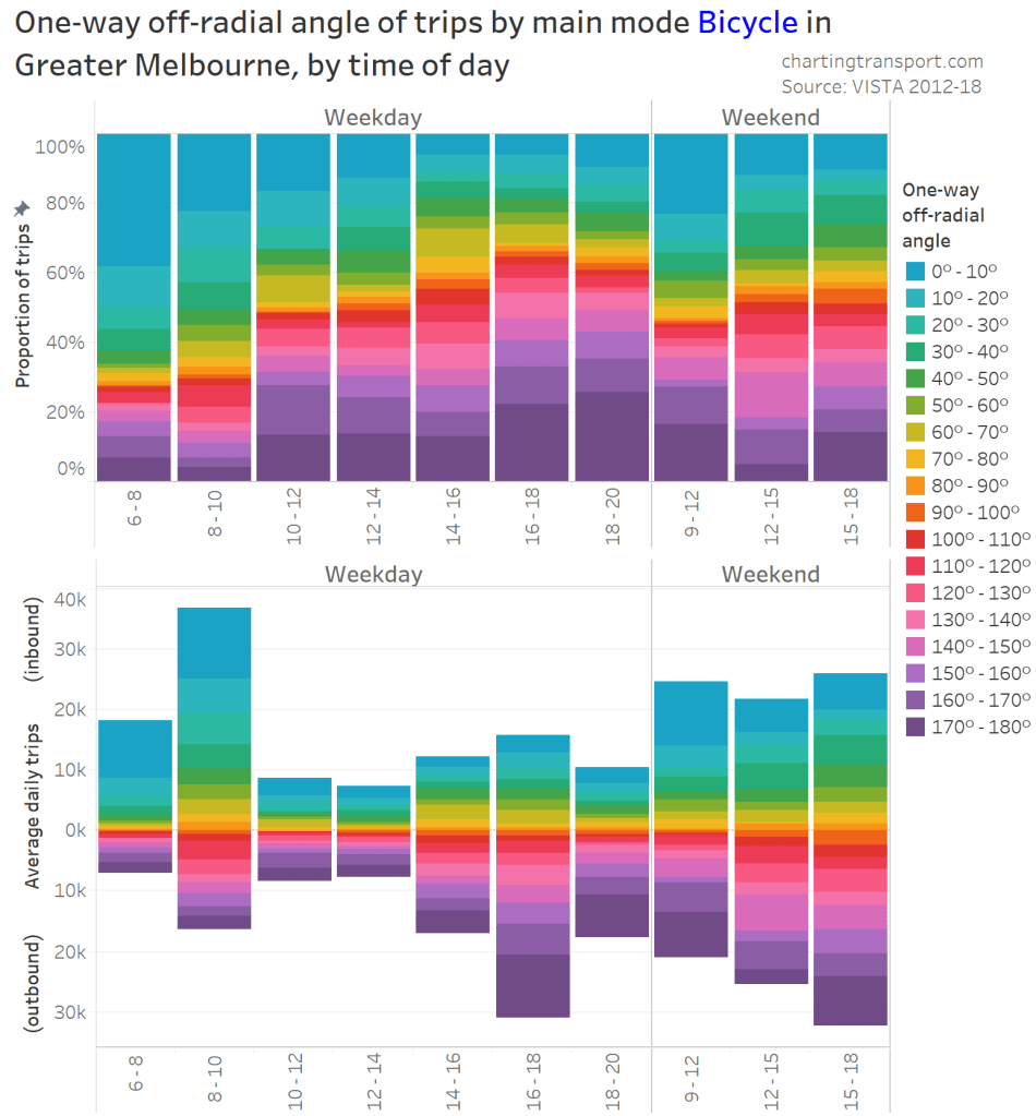
There’s a fair amount of diversity, across the day, with inbound trips dominating the AM peak and outbound trips in the PM commuter peak (but not as strongly in the PM school peak). Weekend late afternoon trips show a little more diversity than morning and early afternoon trips, but the volumes are relatively small.

Next is walking trips:

There is considerable diversity in off-radial angles across most of the week, although outbound trips have a larger share in the late evening.

Walking volumes on weekdays peak at school times. On weekends walking seems to peak between 10 am and 12 pm and again 4 pm to 6 pm, but not considerably compared to the rest of the day time.

Mapping mode shares and radialness

So far I’ve been looking at radialness for modes by time of day. This section next section looks at radialness and mode shares by origins and destinations within Melbourne.

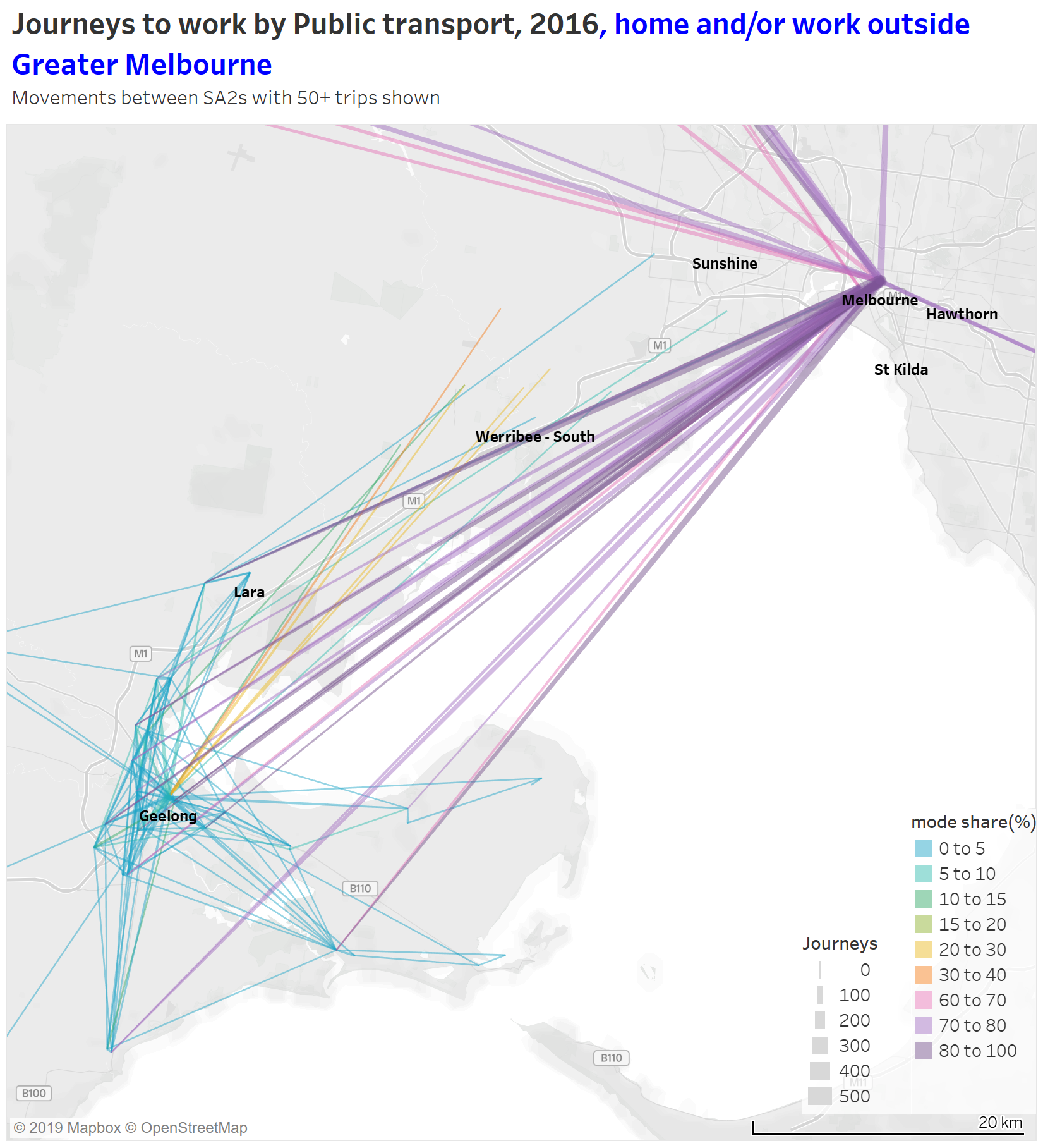
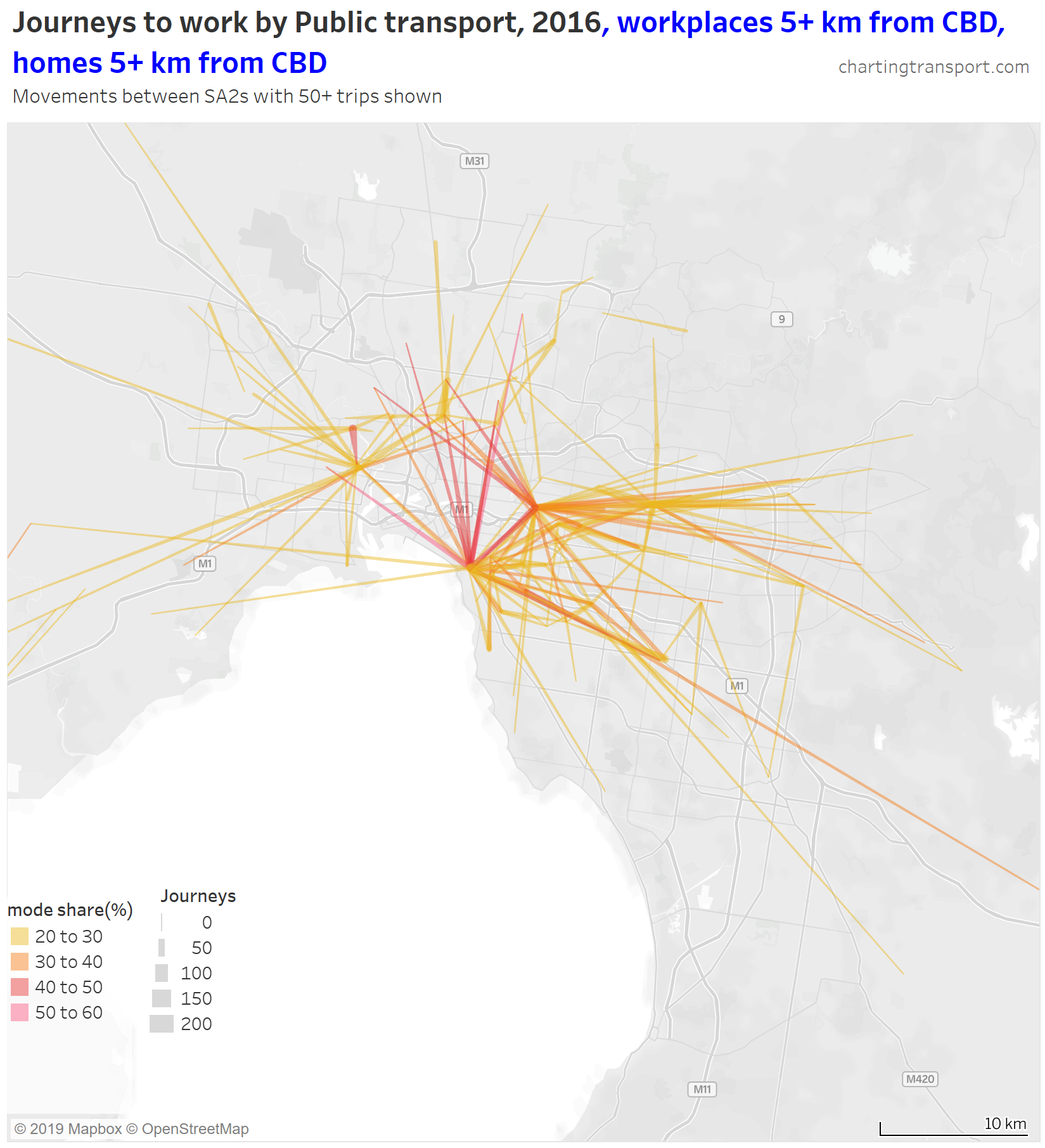
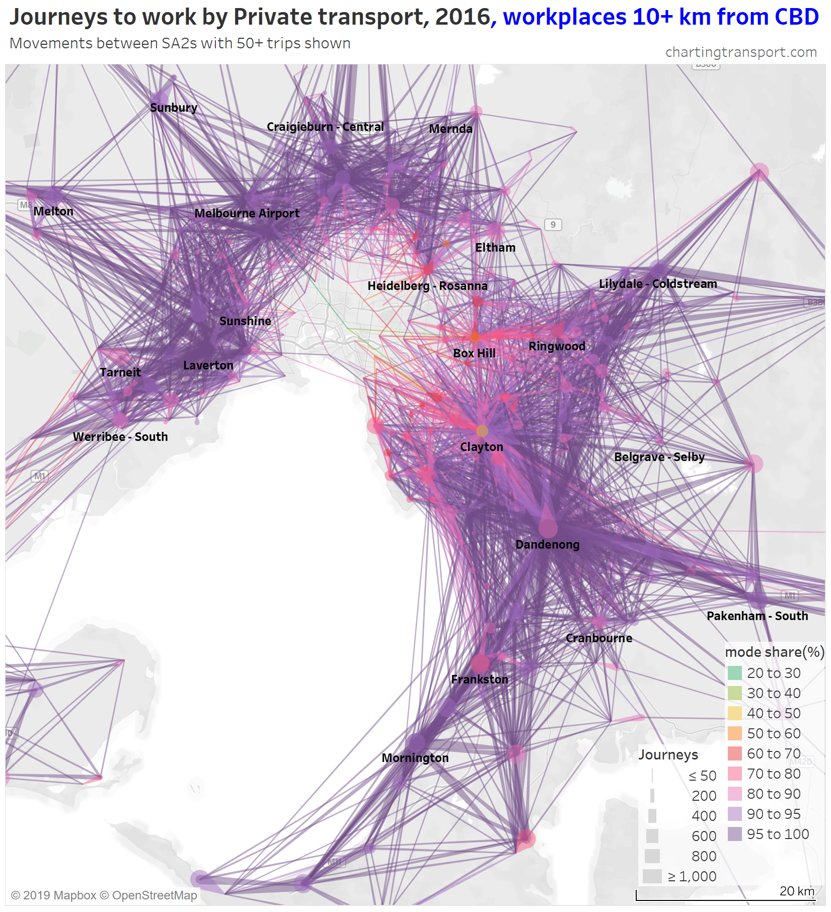
In recent posts I’ve had fun mapping journeys to work from census data (see: Mapping Melbourne’s journeys to work), so I’ve been keep to explore what’s possible for general travel.

VISTA is only a survey of travel (rather than a census), so if you want to map mode shares of trips around the city, you unfortunately need to lose a lot of geographic resolution to get reasonable sample sizes.

The following map shows private transport mode shares for journeys between SA3s (which are roughly the size of municipalities), where there were at least 80 surveyed trips (yes, that is a small sample size so confidence intervals are wider, but I’m also showing mode shares in 10% ranges). Dots indicate trips within an SA3, and lines indicate trips between SA3s. I’ve animated the map to make try to make it slightly easier to call out the high and low private mode shares.

You can see lower private transport mode shares for radial travel involving the central city (Melbourne City SA3), particularly from inner and middle suburbs (less so from outer suburbs). Radial travel that doesn’t go to the city centre generally has high private transport mode shares.

I also have origin and destination SA1s for surveyed trips. Here is a map showing all SA1-SA1 survey trip combinations by main mode, animated to show intervals of two-way off-radial angles:

It’s certainly not a perfect representation because of the all the overlapping lines (I have used a high degree of transparency). You can generally see more blue lines (public transport) in the highly radial angles, and almost entirely red (private transport) and short green lines (active transport) for larger angle ranges. This is consistent with charts in my last post (see: How radial is general travel in Melbourne? (Part 1)).

You can also see that few trips fall into the 80-90° interval, which is because I’m measuring radialness relative to the trip endpoint furthest from the CBD. An angle of 80-90° requires the origin and destination to be about the same distance from the CBD and for the trip to be relatively short.

So there you go, almost certainly more than you ever wanted or needed to know about the radialness of travel in Melbourne. I suspect many of the patterns would also be found in other cities, although some aspects – such the as the geography of Port Phillip Bay – will be unique to Melbourne.

Again, I want to the thank the Department of Transport for sharing the full VISTA data set with me to enable this analysis.


Mapping Melbourne’s journeys to work

Mon 24 June, 2019

The unwritten rules of mapping data include avoiding too much data and clutter, and not using too much colour. This blog often violates those rules, and when it comes to visualising journeys to work, I think we can learn a lot about cities with somewhat cluttered colourful animated maps.

This post maps journeys to work in Melbourne, using data from the 2016 census. I will look at which types of home-work pairs have different public, private and active transport mode shares and volumes.

Although this post will focus on Melbourne, I will include a brief comparison to Sydney at the end.

Where are public transport journeys to work in Melbourne?

First I need to explain the maps you are about to see.

So that I can show mode shares, I’ve grouped journeys between SA2s (which are roughly the size of a suburb). Lines are drawn from the population centroid of the home SA2 (thin end) to the employment centroid of the work SA2 (thicker end). Centroids are calculated as the weighted average location residents/jobs in each SA2 (using mesh block / destination zone data). This generally works okay for urban areas, but be aware that actual trips will be distributed across SA2s, and some SA2s on the urban fringe are quite large.

The thickness of each line at the work end is roughly proportional to the number of journeys by the mode of interest between the home-work pair (refer legends), but it’s difficult to use a scale that is meaningful for smaller volumes. Unfortunately there’s only so much you can do on a 2-D chart.

I’ve not drawn lines where there are fewer than 50 journeys in total (all modes), or where there were no journeys of the mode that is the subject of the map. This threshold of 50 isn’t perfect either as SA2s are not consistently sized within and between cities, so larger SA2s are more likely to generate lines on the map.

To try to help deal with the clutter, I’ve made the lines somewhat transparent, and also animated the map to highlight trips with different mode share intervals. For frames showing all lines, the lines with highest mode share are drawn on top.

So here is an animated map showing public transport journeys to work in Melbourne, by different mode share ranges and overall:

Technical note: I have included journeys to work that are internal to an SA2. Usually these appear as simple circles, but sometimes they appear as small teardrops where the population and employment centroids are sufficiently far apart.

You can see that the highest PT shares and largest PT volumes are for journeys to the central city, and generally from SA2s connected to Melbourne CBD by train (including many outer suburbs).

As the animation moves to highlight lower PT mode share ranges, the lines become a little less radial, a little shorter on average, and the lowest (non-zero) PT mode shares are mostly for suburban trips.

A notable exception is journeys to Port Melbourne Industrial SA2 (also known as Fishermans Bend), which is located at the junction of two major motorways and is remote from rapid public transport (it does however have a couple of high frequency bus lines from the CBD).

The lowest PT mode shares are seen for trips around the outer suburbs. The maps above unfortunately aren’t very good at differentiating small volumes. The following animated map shows public transport journeys with a filter progressively applied to remove lines with small numbers of public transport journeys (refer blue text in title):

You can see that most of the outer suburban lines quickly disappear as they have very small volumes. Inter-suburban lines with more than 50 public transport journeys go to centres including Dandenong, Clayton, Box Hill, and Heidelberg.

Here’s another animation that builds up the map starting with low public transport mode share lines, and then progressively adds lines with higher public transport mode shares:

As an aside, here is a chart showing journeys to work by straight line distance (between SA2 centroids), public transport mode share, work distance from the CBD and home-work volume:

The black dots represent journeys to the inner 5km of the city, and you can see public transport has a high mode share of longer trips. Public transport mode share falls away for shorter journeys to the inner city as people are more likely to use active transport. A dot on the top left of the curve is 8,874 journeys from Docklands to Melbourne – which benefits from the free tram zone and the distances can be 1-2 km. Most of the longer journeys with low public transport mode share are to workplaces remote from the CBD (coloured dots).

Another way to deal with the clutter of overlapping lines around the CBD is to progressively remove lines to workplaces in and around the CBD. Here is another animated map that does exactly so that you can better see journeys in the nearby inner and middle suburbs.

As you strip away the CBD and inner suburbs, you lose most lines with high public transport mode shares and volumes. However some high public transport mode share lines remain, including the following outbound journeys:

  • Melbourne (CBD) to Melbourne Airport: 72% of 64 journeys
  • Melbourne (CBD) to Box Hill: 66% of 76 journeys
  • Melbourne (CBD) to Clayton: 57% of 82 journeys
  • South Yarra – East to Clayton: 57% of 173 journeys

Just keep in mind that these are all very small volumes compared to total journeys in Melbourne.

You might have noticed on the western edge of the map some yellow and orange lines from the Wyndham area (south-west Melbourne) that go off the map towards the south west. These journeys go to Geelong.

Here’s a map showing journeys around Geelong and between Geelong and Greater Melbourne (journeys entirely within Greater Melbourne excluded):

You can see very high public transport mode shares for journeys from the Geelong and Bellarine region to the Melbourne CBD and Docklands (and fairly large volumes), but no lines to Southbank, East Melbourne, Parkville or Carlton – all more remote from Southern Cross Station, the city terminus for regional trains.

(The other purple lines to the CBD are from Ballarat, Bacchus Marsh, Daylesford, Woodend, Kyneton, Castlemaine, Kilmore-Broadford and Warragul, with at least 60 journeys each.)

You can also see those orange and yellow lines from the Wyndham area to central Geelong, being mode shares of 20-40%. The Geelong train line provides frequent services between Tarneit, Wyndham Vale, and Geelong, and has proved reasonably popular with commuters to Geelong (frequency was significantly upgraded in June 2015 with the opening of the Regional Rail Link, just 14 months before the census of August 2016).

However, public transport mode shares for travel within Greater Geelong are very small – even for SA2 that are connected by trains. This might reflect Geelong train station being on the edge of its CBD, relatively cheap parking in central Geelong, limited stopping frequency at some stations (many at 40 minute base pattern), and/or limited walk-up population catchments at several of Geelong’s suburban train stations.

Does public transport have significant mode share for cross-suburban journeys to work?

To search for cross-suburban journeys with relatively high public transport mode shares, here is a map that only shows lines with public transport mode shares above 20% between homes and workplaces both more than 5 km from the CBD (yes, those are arbitrary thresholds):

Of these journeys, the highest mode shares are for journeys from the inner northern suburbs to St Kilda and Hawthorn. There’s also a 49% mode share from Footscray to Maribyrnong (connected by frequent trams and buses).

The tear drop to the north of the city is 114 people who used PT from Coburg to Brunswick (connected by two tram routes and one train route).

Most of the other links on this map are fairly well aligned with train, tram, or SmartBus routes, suggesting high quality services are required to attract significant mode shares.

But these trips are a tiny fraction of journeys to work around Melbourne. In fact 3.0% of journeys to work in Melbourne were by public transport to workplaces more than 5 km from the CBD. The same statistic for Sydney is more than double this, at 7.3%.

What about private transport journeys?

Firstly, here’s a map showing private transport mode shares and volumes, building up the map starting with low private mode share lines.

The links with lowest private transport mode shares are very radial as you might expect (pretty much the inverse of the public transport maps). Progressively less radial lines get added to the map before there is a big bang when the final private transport mode share band of 95-100% gets added, with large volumes of outer suburban trips.

For completeness, here’s an animation that highlights each mode share range individually.

There are some other interesting stories in this data. The following map shows private transport mode share of journeys to work, excluding workplaces up to 10 km from the CBD to remove some clutter.

If you look carefully you’ll see that there is a much lower density of trips that cross the Yarra River (which runs just south of Heidelberg and Eltham). There are limited bridge crossings, and this is probably inhibiting people considering such journeys.

The construction of the North East Link motorway will add considerable cross-Yarra road capacity, and I suspect it may induce more private transport journeys to work across the Yarra River (although tolls will be a disincentive).

What about active transport journeys?

Next is a map for active transport journeys, but this time I’ve progressively added a filter for the number of active transport journeys, as most of the lines on the full chart are for very small volumes.

As soon as the filter reaches a minimum of 50 active journeys most of the lines between SA2s in the middle and outer suburbs disappear. Note that journeys between SA2s are not necessarily long, they might just be a short trip over the boundary.

Then at minimum 200 journeys you can only see central city journeys plus intra-SA2 journeys in relatively dense centres such as Hawthorn, Heidelberg, Box Hill, Clayton, Frankston, Mornington, Footscray, and St Kilda. The large volume in the south of the map that hangs around is Hastings – Somers, where 882 used active transport (probably mostly walking to work on the HMAS Cerebus navy base).

Active transport journeys are mostly much shorter than private and public transport journeys – as you might expect as most people will only walk or ride a bicycle so far. But there are people who said they made very long active transport journeys to work – the map shows some journeys from Point Nepean, Torquay, Ballarat, Daylesford, and Castlemaine to Melbourne. That’s some keen cyclists, incredible runners, people who changed jobs in the week of the census (the census asks for work location the prior week, and modes used on census day), and/or people who didn’t fill in their census forms accurately. The volumes of these trips are very small (mostly less than 5).

That map is very congested around the central city, so here is a map zoomed into the inner suburbs and this time animated by building up the map starting with high active transport mode share lines.

The highest active transport mode shares are for travel within Southbank and from Carlton to Parkville, followed by journeys to places like the CBD, Docklands, South Yarra, South Melbourne, Carlton, Fitzroy, Parkville, and Carlton.

Then you see a lot of trips added from the inner northern suburbs, which are connected to the central city by dare-I-say “above average” cycling infrastructure across some relatively flat terrain. In particular, a thick red line on the map is for 471 active transport journeys from Brunswick to Melbourne (CBD) with a mode share of 17%. A second thick red line is Richmond to Melbourne (CBD) being 589 journeys with 16% active mode share.

Another way of summarising mode shares by work and home distance from the CBD

I’ve experimented with another visualisation approach to overcome the clutter issues. The next charts have home distances from the CBD on the Y axis, work distances from the CBD on the X axis, bubble size representing number of journeys, and colour showing mode shares. I’m drawing smaller journey volumes on top, and I’ve used some transparency to help a little with the clutter.

Firstly here is public transport (animated to show each mode share range individually):

The chart is roughly a V-shape with many trips on the left edge and along a diagonal (mostly representing intra-SA2 journeys), then with several vertical stripes being major suburban employment destinations (including Dandenong at 31 km, Clayton at 19 km, and Frankston at 40 km). Trips above the diagonal are roughly inbound, while trips below the diagonal are roughly outbound.

Some observations:

  • The diagonal line (mostly local journeys) has very low public transport mode shares (sometimes zero).
  • Higher PT mode shares are only seen on the far left and bottom left hand corner of the chart. Some outliers include Richmond to Box Hill (32%), Clayton to Malvern East (32%), and South Yarra – East to Clayton (57%).
  • PT mode shares of 80+% are only seen for journeys to the CBD from home SA2s at least 11 km out (with one exception of Melbourne CBD to St Kilda with 80% PT share).
  • Home-work pairs with zero public transport journeys are scattered around the middle and outer suburbs, most being longer distance journeys (home and work at different distances from the CBD).

Here’s the same chart for private transport:

The lowest private transport shares are seen for journeys to the CBD. The diagonal has many mode shares in the 80-90% range.

And here is active transport:

The highest active transport mode shares are seen in the central city area, followed by the diagonal mostly representing local journeys (with generally higher shares closer to the CBD). Some notable outliers include local trips within Clayton (1,298 active trips / 46% active mode share), Box Hill (914 / 40%), Hastings – Somers (1,762 / 27%), Flinders (240 / 24%), Glen Waverley – West (308 / 21%), and Mentone (226 / 23%).

How does Sydney compare to Melbourne?

Here is a chart with private transport mode share maps for both Melbourne and Sydney, animated in tandem to progressively add higher mode share journeys.

You can see that Sydney has a lot more trips at lower private transport mode shares, and that workplaces outside the city centre start to show up earlier in the animation in Sydney – being the dense transit-orientated suburban employment clusters that are largely unique to Sydney (see: Suburban employment clusters and the journey to work in Australian cities).

If time permits, I may do similar analysis for Sydney and other cities in future posts.


How radial are journeys to work in Australian cities?

Fri 14 June, 2019

In almost every city, hordes of people commute towards the city centre in the morning and back away from the city in the evening. This largely radial travel causes plenty of congestion on road and public transport networks.

But only a fraction of commuters in each city actually work in the CBD. So just how radial are journeys to work? How does it vary between cities? And how does it vary by mode of transport?

This post takes a detailed look at journey to work data from the ABS 2016 Census for Melbourne, Sydney, and to a less extent Brisbane, Perth, Adelaide and Canberra. I’ve included some visualisations for Melbourne and Sydney that I hope you will find interesting.

How to measure radialness?

I’m measuring radialness by the difference in degrees between the bearing of the journey to work, and a direct line from the home to the CBD of the city. I’m calling this the “off-radial angle”.

So an off-radial angle of 0° means the journey to work headed directly towards the CBD. However that doesn’t mean the workplace was the CBD, it might be have been short of the CBD or even on the opposite side of the CBD.

Similarly, an off-radial angle of 180° means the journey to work headed directly away from the CBD. And a value of 90° means that the trip was “orbital” relative to the CBD (a Melbourne example would be a journey from Box Hill that headed either north or south). And then there are all the angles in between.

To deal with data on literally millions of journeys to work, I’ve grouped journeys by home and work SA2 (SA2s are roughly the size of a suburb), and my bearing calculations are based on the residential centroid of the home SA2 and the employment centroid of the work SA2.

So it is certainly not precise analysis, but I’ve also grouped off-radial angles into 10 degree intervals, and I’m mostly looking for general trends and patterns.

So how radial are trips in Melbourne and Sydney?

Here’s a chart showing the proportion of 2016 journeys to work at different off-radial angle intervals:

Technical note: As per all my posts, I’ve designated a main mode for journeys to work: any journey involving public transport is classed as “Public”, any journey not involving motorised transport is classed as “Active”, and any other journey is classed as “Private”.

In both cities over 30% of journeys to work were what you might call “very radial” – within 10 degrees of perfectly radial. It was slightly higher in Melbourne.

You can also see that public transport trips are even more radial, particularly in Melbourne. In fact, around two-thirds of public transport journeys to work in 2016 had a destination within 2 km of the CBD.

Melbourne’s “mass transit” system (mostly trains and trams) is very radial, so you might be wondering why public transport accounts for less than half of those very radial journeys (41% in fact).

Here are Melbourne’s “very radial” journeys broken down by workplace distance from the Melbourne CBD:

very-radial-trips-by-mode-distance-from-cbd

Public transport dominates very radial journeys to workplaces within 2 km of the centre of the CBD, but is a minority mode for workplaces at all other distances. Many of these highly radial journeys might not line up with a transit line towards the city, and/or there could well be free parking at those suburban workplaces that make driving all too easy. I will explore this more shortly.

Sydney however had higher public transport mode shares for less radial journeys to work. I think this can be explained by Sydney’s large and dense suburban employment clusters that achieve relatively high public transport mode shares (see: Suburban employment clusters and the journey to work in Australian cities), the less radial nature of Sydney’s train network, and generally higher levels of public transport service provision, particularly in inner and middle suburbs.

Visualising radialness on maps

To visualise journeys to work it is necessary to simplify things a little so maps don’t get completely cluttered. On the following maps I show journey to work volumes between SA2s where there are at least 50 journeys for which the mode is known. The lines between home and work SA2s get thicker at the work end, and the thickness is proportional to the volume (although it’s hard to get a scale that works for all scenarios).

First up is an animated map that shows journeys to work coloured by private transport mode share, with each frame showing a different interval of off-radial angle (plus one very cluttered view with all trips):

(click/tap to enlarge maps)

I’ve had to use a lot of transparency so you have a chance at making out overlapping lines, but unfortunately that makes individual lines a little harder to see, particularly for the larger off-radial angles.

You can see a large number of near-radial journeys, and then a smattering of journeys at other off-radial angles, with some large volumes across the middle suburbs at particular angles.

The frame showing very radial trips was rather cluttered, so here is an map showing only those trips, animated to strip out workplaces in the CBD and surrounds so you can see the other journeys:

Private transport mode shares of very radial trips are only very low for trips to the central city. When the central city jobs are stripped out, you see mostly high private transport mode shares. Some relative exceptions to this include journeys to places like Box Hill, Hawthorn, and Footscray. More on that in a future post.

Here are the same maps for Sydney:

Across both of these maps you can find Sydney’s suburban employment clusters which have relatively low private transport mode shares. I explore this, and many other interesting ways to visualise journeys to work on maps in another post.

What about other Australian cities?

To compare several cities on one chart, I need some summary statistics. I’ve settled on two measures that are relatively easy to calculate – namely the average off-radial angle, and the percent of journeys that are very radial (up to 10°).

The ACT (Canberra) actually has the most radial journeys to work of these six cities, despite it being something of a polycentric city. Adelaide has the next most radial journeys to work, but there’s not a lot of difference in the largest four cities, despite Sydney being much more a polycentric city than the others. Note the two metrics do not correlate strongly – summary statistics are always problematic!

Here are those radialness measures again, but broken down by main mode:

Sydney now looks the least radial of the cities on most measures and modes, particularly by public transport.

The Australian Capital Territory (Canberra) has highly radial private and active journeys to work, but much less-radial public transport journeys than most other cities. This probably reflects Canberra’s relatively low cost parking (easy to drive to the inner city), but also that the public transport bus network is orientated around the suburban town centres that contain decent quantities of jobs.

Adelaide has the most radial journeys to work when it comes to active and public transport.

What about other types of travel?

In a future post, I’ll look at the radialness of general travel around Melbourne using household travel survey data (VISTA), and answer some questions I’ve been pondering for a while. Is general travel around cities significantly less radial than journeys to work? Is weekend travel less radial than weekday travel?

Follow the blog on twitter or become an email subscriber (see top-right of this page) to get alerted when that comes out.


Visualising the components of population change in Australia

Sat 27 April, 2019

Australian cities are growing in population as a result of international migration, internal migration, and births outnumbering deaths. But which of these factors are most at play in different parts of the country?

Thanks to ABS publishing data on the components of population growth with their Regional Population Growth product, we now have estimates of births, deaths, internal/international arrivals, and internal/international departures right down to SA2 geography for 2016-17 and 2017-18.

This post aims to summarise the main explanation for population change in different parts of the country.

This post isn’t much about transport, but I hope you also find the data interesting. That said, it’s possible that immigrants from transit-orientated countries might be more inclined to use public transport in Australia, and that might impact transport demand patterns. We know that recent immigrants are more likely to travel to work by public transport than longer term residents, but that probably also has a lot to do with where they are settling.

How is population changing in bigger and smaller cities?

First up, I’ve divided Australia into Capital Cities (Greater Capital City Statistical Areas), Large regional cities (Significant Urban Areas with population 100,000+, 2016 boundaries), small regional cities (Significant Urban Areas, with population 10,000 to 100,000, 2016 boundaries ) and “elsewhere”.

Here’s a chart showing the total of the six components of population change in each of those four place types. I’ve animated the chart (and most upcoming charts) to show changes in the years to June 2017 and June 2018, with a longer pause on 2018.

There were significant internal movements in all parts of Australia (shown in green) – even more so in 2018. These include people moving between any SA2s, whether they adjacent within a city or across the country.

International arrivals and departures were much larger in capital cities and there were more arrivals than departures in all four place types. International arrivals declined between 2017 and 2018, while international departures increased slightly between 2017 and 2018.

Births also outnumbered deaths in all place categories in both years.

Here’s a look at the larger capital cities individually:

The chart shows Sydney, Perth, and Adelaide had more internal departures than arrivals. These cities only grew in total population because of natural increase and net international immigration. Melbourne and Brisbane had a net increase from internal movements in both 2017 and 2018, while Canberra has been a lot more even.

International arrivals outnumbered international departures and births significantly outnumbered deaths in all cities. Melbourne and Canberra were the only cities to see a significant increase in international arrivals between 2017 and 2018.

Here is the same chart but for medium sized cities:

Again, there were much larger volumes of internal migration in 2017-18 compared to 2016-17.

The Gold Coast is the only medium-sized city to have significant volumes of international movements. The fast population growth of the Gold and Sunshine Coasts is mostly coming from internal arrivals.

What is the dominant explanation for population change in different parts of Australia?

As mentioned the ABS data goes down to SA2 statistical geography which allows particularly fine grain analysis, with six measures available for each SA2. However it is difficult to show those six components spatially. They can be consolidated into three categories: net natural increase, net internal arrivals/departures, and net international arrivals/departures, but that is still three different metrics for all SA2s.

One way to look at this is simply the component with the largest contribution to population growth (or decline). Here is a map showing that for each SA2 in Melbourne:

You can see that international arrivals dominated population growth in most inner and middle suburbs, while internal arrivals dominated population growth in most outer suburbs. There are also some SA2s where births dominated (often low growth outer suburbs).

This representation is quite simplified, and doesn’t show what else might be happening. For example, here is a summary of the population changes in Sunshine for the year to June 2018:

Population change in Sunshine, year to June 2018

Overseas arrivals dominated population growth (net +313), but the otherwise hidden story here is that they were largely offset by net internal departures of 279.

So to add more detail to the analysis, I’ve created a slightly more detailed classification system that looks at the largest component and often a secondary component, as per the following table.

Explanation summaryLargest componentOther components
Growth – mostly births replacing localsNatural increaseNet internal departures more than 50 and net internal departures more than net overseas departures
Growth – mostly birthsNatural increaseNet internal and overseas departures of no more than 50
Growth – mostly immigrants replacing localsNet overseas arrivalsNet internal departures of at least 50 and/or natural decrease of at least 50.
Growth – mostly immigrationNet overseas arrivalsNet internal departures less than 50 (or net arrivals).
Growth – mostly internal arrivals replacing deathsNet internal arrivalsNet natural decrease of 50 or more, and bigger than net overseas departures
Growth – mostly internal arrivalsNet internal arrivalsNet internal arrivals greater than net overseas arrivals and natural increase

Decline – mostly internal departures

Net internal departures

Natural increase and net overseas arrivals both less than 50
Decline – mostly internal departures partly offset by births Net internal departuresNatural increase of at least 50, and natural increase larger than net overseas arrivals.
Decline – mostly internal departures partly offset by immigrantsNet internal departures Net overseas arrivals of at least 50, and net overseas arrivals larger than natural increase.
Decline – mostly deathsNatural decrease

There are no SA2s where net international departures was the major explanation for population change.

Here’s what these summary explanations look like in Melbourne (again, animated to show years to June 2017 and June 2018):

Technical notes: On these maps I’ve omitted SA2s where there was population change of less than 50 people, or where no components of population change were more than 1% of the population. Not all classifications are present on all maps.

You can now see that in most middle suburbs there has been a net exodus of locals, more than offset by net international arrivals (light purple). Also, many of the outer suburbs with low growth actually involve births offsetting internal departures (light blue).

Turning near-continuous data into discrete classifications is still slightly problematic. For example the summary explanations don’t tell you by how much one component was larger than the others. For example if there were 561 net international arrivals and 560 net internal arrivals, it would be classified as “Growth – mostly immigration”. Also, SA2s are not consistently sized across Australia (see: How is density changing in Australian cities?), so my threshold of 50 is not perfect. At the end of the post I provide a link to Tableau where you can inspect the data more closely for any part of Australia.

The inner city area of Melbourne was a little congested with data marks on the above map, so here is a map zoomed into inner and middle Melbourne:

You can see significant population growth in the Melbourne CBD and surrounding SA2s, particularly in 2017. The main explanation for inner city growth is international immigration, although internal arrivals came out on top in Southbank in 2018. Curiously, net internal arrivals were larger the international migration in Brunswick East in both years. And natural increase was dominant in Newport in the inner-west.

Zooming out to include the bigger regional centres of Victoria (note: many regional SA2s don’t show up because of very little population change):

In most regional Victorian cities, internal arrivals account for most of the population growth, although the net growth in “Shepparton – North” of +222 in 2017 and +152 in 2018 was mostly made up of international arrivals.
The only other SA2s to show international arrivals as the main explanation were in inner Geelong.

(I haven’t shown all of Victoria because few SA2s outside the above map had significant population change).

Heading up to Sydney, the picture is fairly similar to Melbourne:

Like Melbourne, internal arrivals accounted for most of the population growth in outer growth areas.

International immigration dominated the inner and middle suburbs in 2017, but in 2018 immigration eased off, and births became the main explanation for population growth in more SA2s.

The middle SA2s of Homebush Bay – Silverwater and Botany are noticeable exceptions to the pattern, dominated by internal arrivals.

Zooming out to New South Wales:

Central Newcastle, central Wollongong, Armidale and Griffith saw mostly international immigration led population growth. Most larger regional towns saw growth from internal arrivals, but further inland there was population decline – mostly from internal departures.

Next up, Brisbane:

Population growth in Brisbane’s inner suburbs is much more of a mix of internal and overseas arrivals. There are also more SA2s where births dominate population growth. There were also some SA2s with slight population decline for various reasons.

Zooming out to South East Queensland:

International arrivals dominated areas on the Gold Coast closer to the coastline, but much less so on the Sunshine Coast and in Toowoomba.

Looking at other parts of Queensland:

There was population decline in several areas, including Mackay and Mount Isa. Rockhampton and Cairns saw population growth mostly through internal arrivals. Townsville was dominated by internal arrivals in 2017, and births in 2018.

Airlie – Whitsundays stands out as having population growth mostly from international arrivals in both years.

Next up, Perth:

Like other cities, population growth in the outer suburbs was dominated by internal arrivals. There were a lot more SA2s showing population decline, and this was largely due to internal departures, partly offset by natural increases or net overseas arrivals.

Zooming out to Western Australia:

Population growth on the south-west coast was mostly dominated by internal arrivals, while in many other centres around the state there was population decline, mostly due to internal departures, however in many areas this was offset partly by births.

Next up, Adelaide:

Firstly, keep in mind that there has been relatively slow population growth in Adelaide (the scale is adjusted). The inner and middle suburbs mostly show population growth from international arrivals (often offsetting net internal departures), and the outer growth areas were again mostly about internal arrivals.

Zooming out to South Australia:

In 2017 there was considerable population decline in Whyalla and Port Augusta. Murray Bridge is another rare regional centre where population growth was largely driven by almost 400 overseas arrivals each year.

Next is Tasmania:

Note the circle size scale is even smaller. Overseas arrivals dominated population growth in central Hobart and Newman – Mayfield in Launceston (possibly related to university campuses), while internal migration dominated most other areas.

Here is Canberra:

International immigrants dominated population growth around Civic and the inner north. Internal arrivals dominated Kingston and Griffith and most outer growth areas. The outer suburbs saw a mixture of births and internal arrivals as the dominant explanation.

And finally, Darwin, which actually saw net population decline in the year to June 2018:

Palmerston South saw the largest population growth – mostly from internal arrivals. International arrivals were significant around Darwin city in 2017, but were much less significant in 2018. Most of the northern suburbs saw population decline in the year to June 2018.

Didn’t see your area, or want to explore further? You can view this data interactively in Tableau (you might want to filter by state as that will change the scale of circle sizes).

Where were international arrivals most significant?

I’ve calculated the ratio of international arrivals to population for each SA2. The SA2s where international arrivals in the year to June 2018 make up a significant portion of the 2018 population are all near universities and/or CBDs. Namely:

  • Melbourne CBD and neighbouring Carlton at 20% (Melbourne Uni, RMIT, and others)
  • Brisbane CBD at 18% and neighbouring Spring Hill at 20% (QUT and others)
  • Clayton in Melbourne at 18% (Monash Uni)
  • Sydney – Haymarket – The Rocks at 15% and neighbouring Pyrmont – Ultimo at 17% (near to UTS, Sydney Uni, and various others)
  • Acton (ACT) at 17% (ANU)
  • Kingsford (in Sydney) at 16% (UNSW)
  • St Lucia (Brisbane) at 15% (UQ)

I hope you’ve found this interesting. In a future post I might look at internal migration origin-destination flows, including how people are moving within and between cities.