This detailed post from 2023 does not include the population latest data. For the latest summary metrics, see Trends in major city population density.
With the release of more detailed 2021 census data and June 2022 population estimates, it’s now possible to look more closely at how Australia’s larger capital cities have changed, particularly following the onset of the COVID19 pandemic in 2020.
This post examines ABS population grid data for 2006 to 2023 for Greater Capital City Statistical Areas, including:
- Trends in overall population-weighted density for cities;
- Changes in the distribution of population living at different densities;
- Changes in the distribution of population living at different distances from each city’s CBD;
- Changes in population density by distance from each city’s CBD;
- Changes in the distribution of population living at different distances from train and busway stations;
- Changes in population density in areas close to train and busway stations;
- The population density of “new” urban residential areas in each city (are cities sprawling at low density?); and
- Changes in the size of the urban residential footprint of cities.
I’ve also got some animated maps showing the density of each city over those years, and I’ve had a bit of a look at how the ABS corrected population estimates for 2007 to 2021 following the release of 2021 census data.
For some other detailed analysis – and a longer history of city population density – see How is density changing in Australian cities? (2nd edition).
I’ve not included the smaller cities of Hobart and Darwin as they have a small footprint, and too many grid cells are on the edge of an urban area.
Population weighted density
My preferred measure of city density is population-weighted density, which takes a weighted average of the density all statistical areas in a city, with each area weighted by its population (this stops lightly populated rural areas pulling down average density – for more discussion see How is density changing in Australian cities? (2nd edition)).
I also prefer to calculate this measure on a consistent statistical area geography and the only consistent statistical area geography available for Australia is the square kilometre population grid published by the ABS.
With the recent release of 2021 census data, ABS issued revised population grid estimates for all years from 2017 onwards, which saw significant corrections in some cities (see appendix for more details). There has also been a slight change in the methodology for the 2021 grid that ABS say may result in a more ‘targeted representation’, but it’s unclear what that means.
Here’s the revised trend in population weighted density calculated on square km grid geography for Greater Capital City Statistical Areas in June of each year:
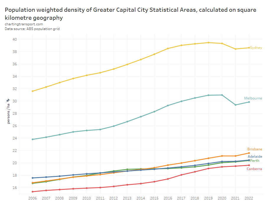
Sydney has almost double the population density of most other Australian cities (on this measure), with the exception being Melbourne which sits halfway in between.
Population weighted density was rising in all cities until 2019, although the growth was notably slowing in Sydney from about 2016.
The pandemic hit in March 2020 and led to a flatlining of density in Melbourne and a decline in Sydney by June 2020, while other cities continued to densify. Then Sydney and Melbourne’s population weighted density dropped considerably in the year to June 2021 – probably a combination an exodus of temporary international migrants and internal migration away from the big cities (particularly Melbourne that had experienced long lockdowns). Most other cities flatlined between June 2020 and June 2021.
Then by June 2022 density had increased again in all cities, after international borders reopened in early 2022.
I expect some fairly substantial changes between June 2022 and June 2023 in some cities as migration has surged further and rental vacancy rates have plummeted in several cities.
Population living at different densities
The following chart shows the proportion of the population in each city living at different density ranges over time:

All cities show a sustained pre-pandemic trend towards more people living at higher densities. However the pandemic saw significant drops in people living at the higher density categories in 2021 in Melbourne, Sydney, and Canberra.
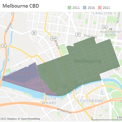
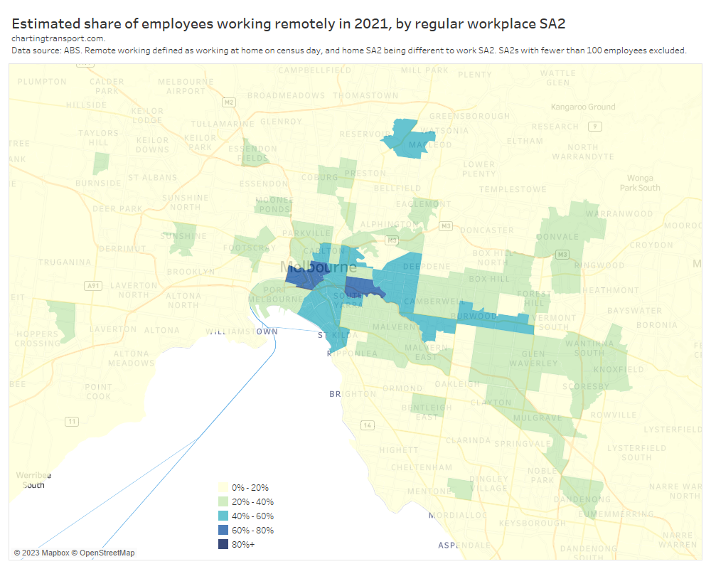
So where was this loss of density? The next chart shows the change in population for grid squares across Melbourne between June 2020 and June 2021. Larger dots are more change, blue is an increase and orange is a decline:
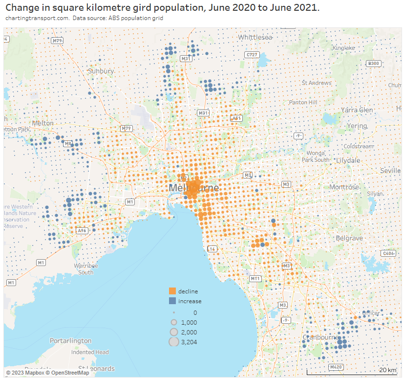
You can see significant declines in population (and hence population density) in the inner city areas – so much so that the dots overlap. This is likely largely explained by the exodus of many international students and other temporary migrants.
You can also see population decline around Monash University’s Clayton campus in the south-eastern suburbs.
At the same time there were large increases in population in the outer growth areas, as is normally the case. Other pockets of population growth include Footscray, Moonee Ponds, Box Hill, Port Melbourne, Clayton (M-City), and Doncaster, likely related to the completion of new residential towers.
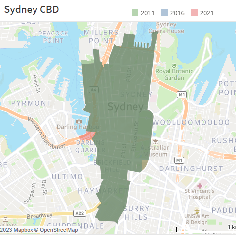
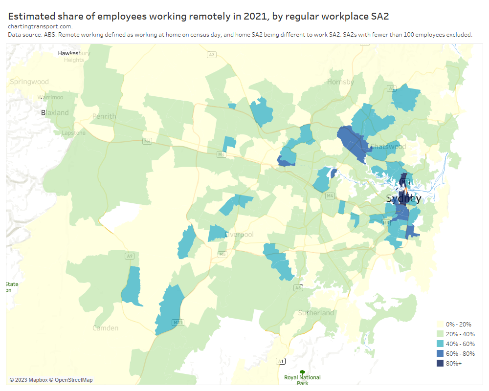
Here’s the same for Sydney:
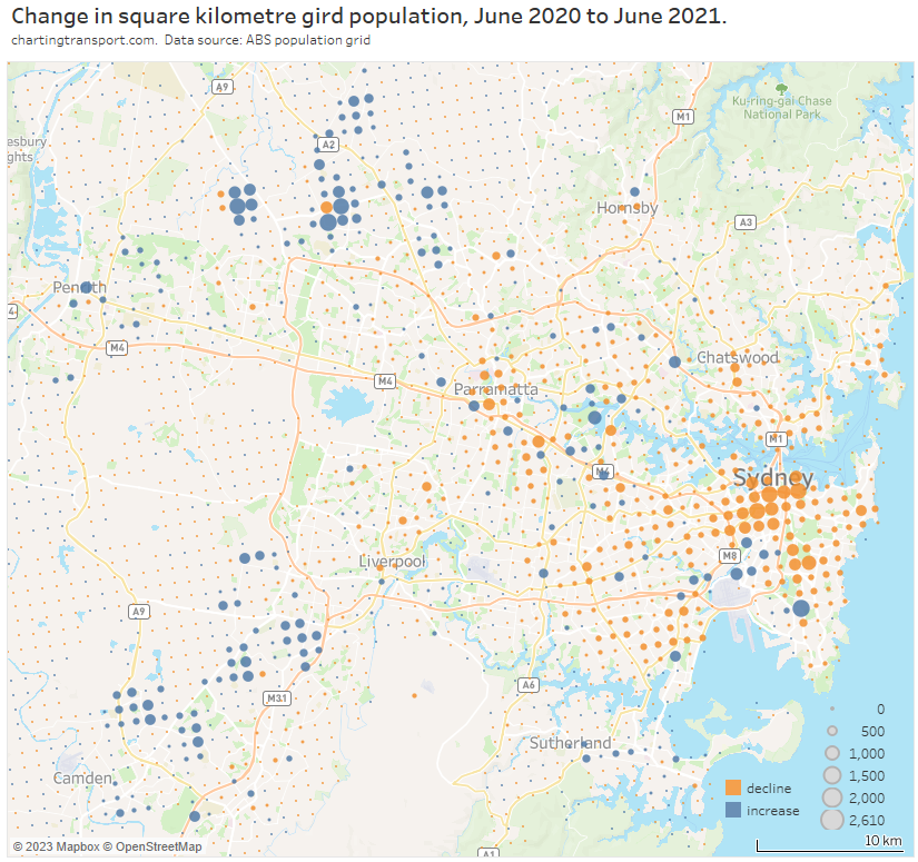
There was significant population decline in the inner city and around Kensington (which has a major university campus), and the largest growth was seen in urban fringe growth areas to the north-west and south-west. Pockets of population growth were also seen at Wentworth Point, Eastgardens, Mascot, North Ryde, and Mays Hill, amongst others.
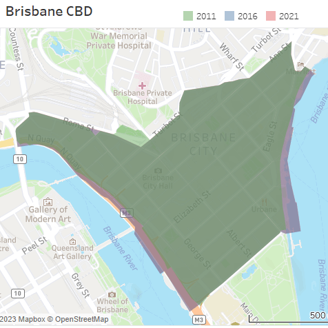
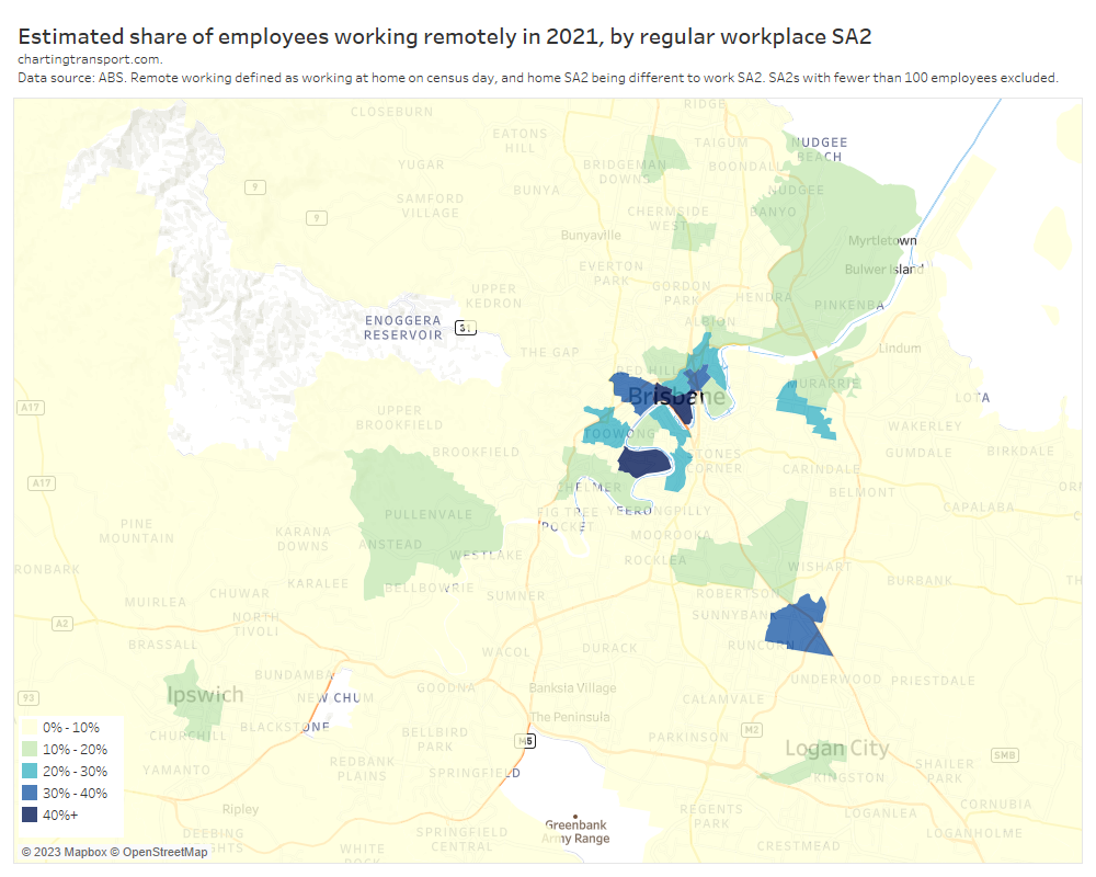
Here is the same for Brisbane:
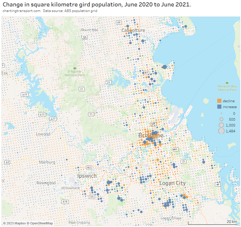
Inner-city Brisbane was much more a mixed bag, which explains the less overall change in the density composition of the city. Some areas showed declines (including St Lucia, New Farm, Kelvin Grove, Coorparoo) while others saw increases (including Fortitude Valley, West End, South Brisbane, Buranda, CBD south).
Proportion of population living at different distances from the city centre
The next chart shows the proportion of people living at approximate distance bands from each city’s CBD over time:
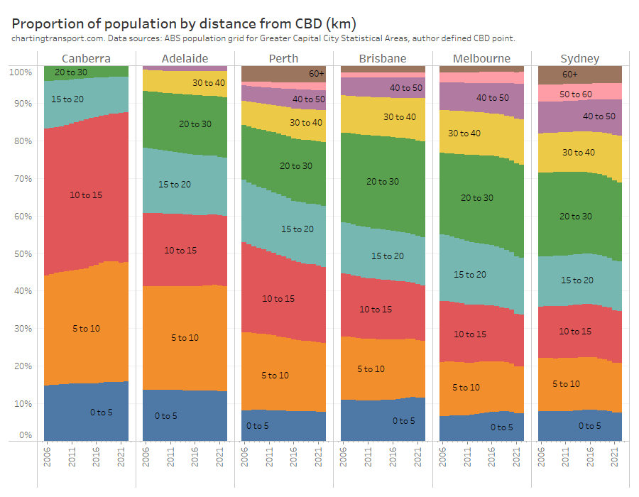
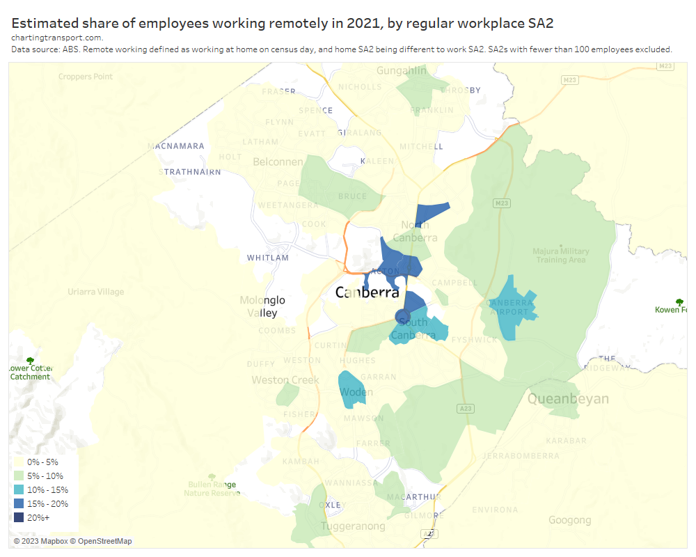
All cities have seen a general trend towards more of their population living further from the CBD, with the notable exception of Canberra which has seen the outer urban fringe expanding by little more than a couple of kilometres at the most, and substantial in-fill housing at major town centres and the inner city (see also animated density map below). I should note that the Greater Capital City Statistical Area boundary for Canberra is simply the ACT boundary, and does not include the neighbouring NSW urban area of Queanbeyan, which is arguably functionally part of “greater Canberra”.
In 2021, Sydney and Melbourne saw a step change towards living further out, in line with the sudden reduction in central city population.
Population density by distance from a city’s CBD
Here’s an animated chart showing how population weighted density has varied by distance from each city’s CBD over time:
In most cities there has been a trend to significantly increasing density closer to the CBD, with central Melbourne overtaking central Sydney in 2017.
Sydney has maintained significantly higher density than all other cities at most distances from CBDs, with Melbourne a fair step behind, then most other cities flatten out to around 20-26 persons/ha from around 6+km out from their CBDs in 2022.
Canberra appears to flatten out to around 20 persons/ha at 3-4 kms from its CBD (Civic) however it is important to note that Canberra has a lot of non-residential land relatively close to Civic which reduces density for many grid cells that are on an urban fringe (refer maps toward the end of this post).
Population living near rapid transit stations
I’ve been maintaining a spatial data set of rapid transit stations (train and busway stations) including years of opening and closing, and from this it’s possible to assess what proportion of each city lives close to stations:
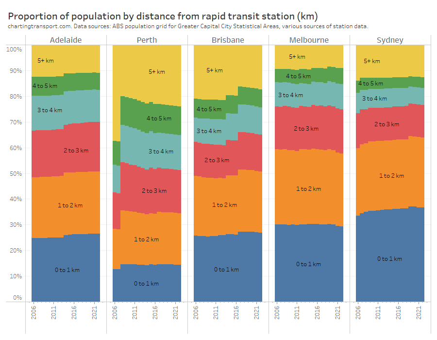
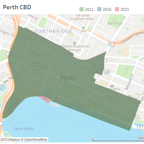
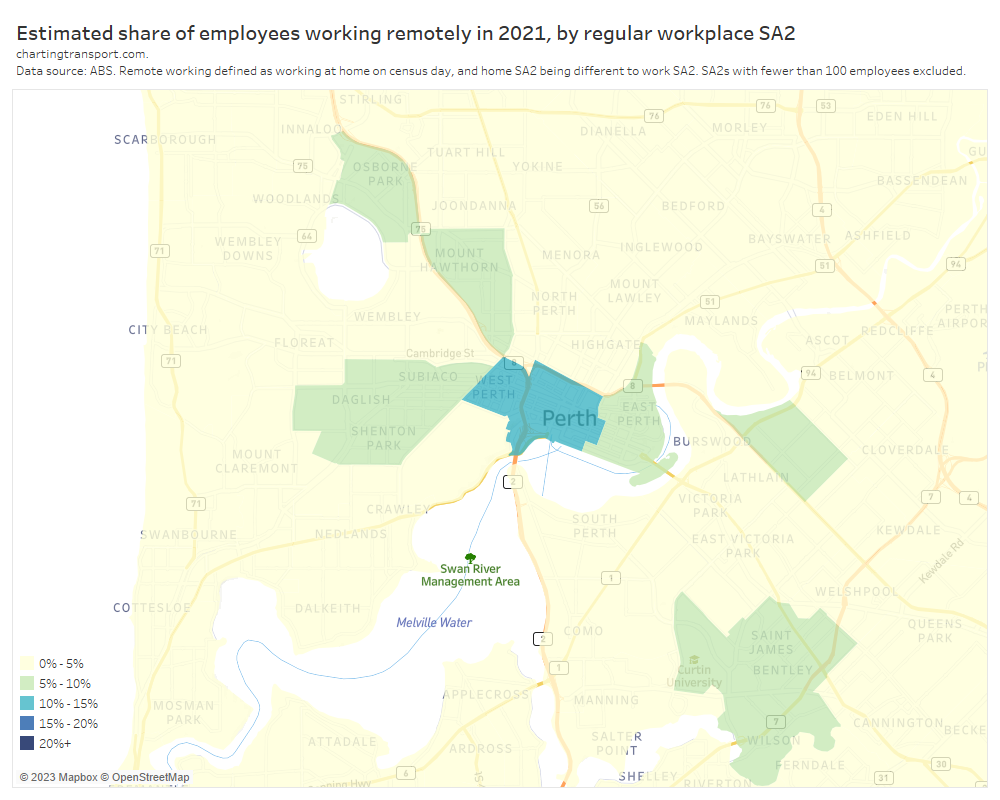
Sydney has the largest proportion of it’s population living quite close to rapid transit stations, with Perth having the lowest.
There are step changes on this chart where new train lines have opened. Sydney, Brisbane, and Adelaide have been successful at increasing population close to stations. The opening of the Mandurah rail line made a big difference in Perth in 2009 but the city has been growing remote from stations since then (MetroNet projects will probably turn this around significantly in the next few years). Melbourne was roughly keeping the same proportion of the population close to stations although that changed in 2021 with the exodus of inner city residents (I anticipate a substantial correction in 2023).
Population density around rapid transit stations
The following animated chart shows the aggregate population-weighted density for areas around rapid transit stations in the five biggest cities over time:

Sydney has lead Australia with higher densities around train stations, followed by Melbourne. Perth has only slightly higher densities around stations (in aggregate) compared to other parts of the city. Population density is generally lower around Adelaide train and busway stations compared to the rest of the city – the antithesis of transit orientated development.
How dense are new urban areas?
I’ve previously looked at the density of outer urban growth areas on my blog, and here is another way of looking at that using square kilometre grid data.
I’ve attempted to identify new urban residential grid squares by filtering for squares that averaged less than 5 persons per hectare in 2006 and more than 5 persons per hectare in 2022 (using 5 persons/ha as an arbitrary threshold for urban residential areas, and I think that’s a pretty low threshold).
The vast bulk of these grid cells (and associated population) are on the urban fringe, but a handful in each city are brownfield sites that were previously non-residential (for Melbourne 99% of the population of these grid cells are in urban fringe areas).
It’s also not perfect because square kilometre grid cells will often contain a mix of residential and non-residential land uses, but it is analysis that can be done easily and quickly, and in aggregate I expect it will be broadly indicate of overall patterns.
The following chart shows the population of new urban residential grid cells (since 2006), and the proportion of this population by 2022 population density:
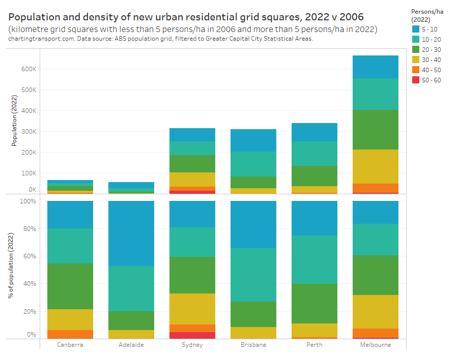
You can see Melbourne has almost double the population in these new urban residential grid squares compared to Perth, Brisbane, and Sydney. This indicates Melbourne has been sprawling more than any other city since 2006. Slow-growing Adelaide only put on about 56k people in new urban grid squares, slightly less than Canberra.
The bottom half of the chart shows that new urban grid squares in Sydney, Melbourne, and Canberra are generally much more dense than those in other cities. This likely reflects planning policies for higher residential densities in new urban areas in those cities. In fact, all of these grid cells with density 40+ in 2022 are on the urban fringes, except one brownfield cell in Mascot (Sydney).
But of course planning policies can change over time, so here is the equivalent chart looking at new urban residential squares since 2012:
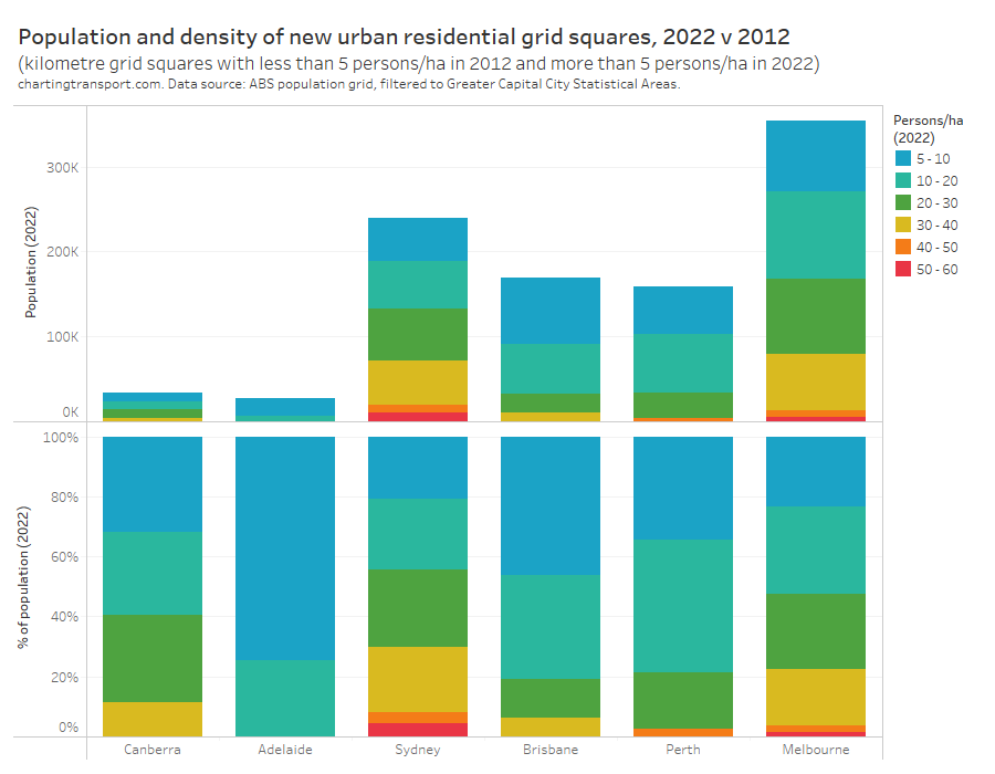
It’s not a lot different. The density of these more recent new urban residential grid cells is generally highest in Sydney, following by Melbourne and Canberra. New urban residential grid cells in Adelaide mostly had fewer than 20 persons/ha, but then also there are not that many such grid cells and they didn’t have much population in 2022.
Perth has managed one new grid cell with over 40 persons/ha in 2022 – it is located in Piara Waters (which has many single storey houses with tiny backyards).
How much has the urban footprint of cities been expanding?
The population grid data only measures residential population so it cannot be used to estimate the size of the total urban footprint of cities over time, but we can use it to estimate the urban residential footprint. I’ve again used 5 persons/ha as a threshold, and here’s how the cities have growth since 2006:
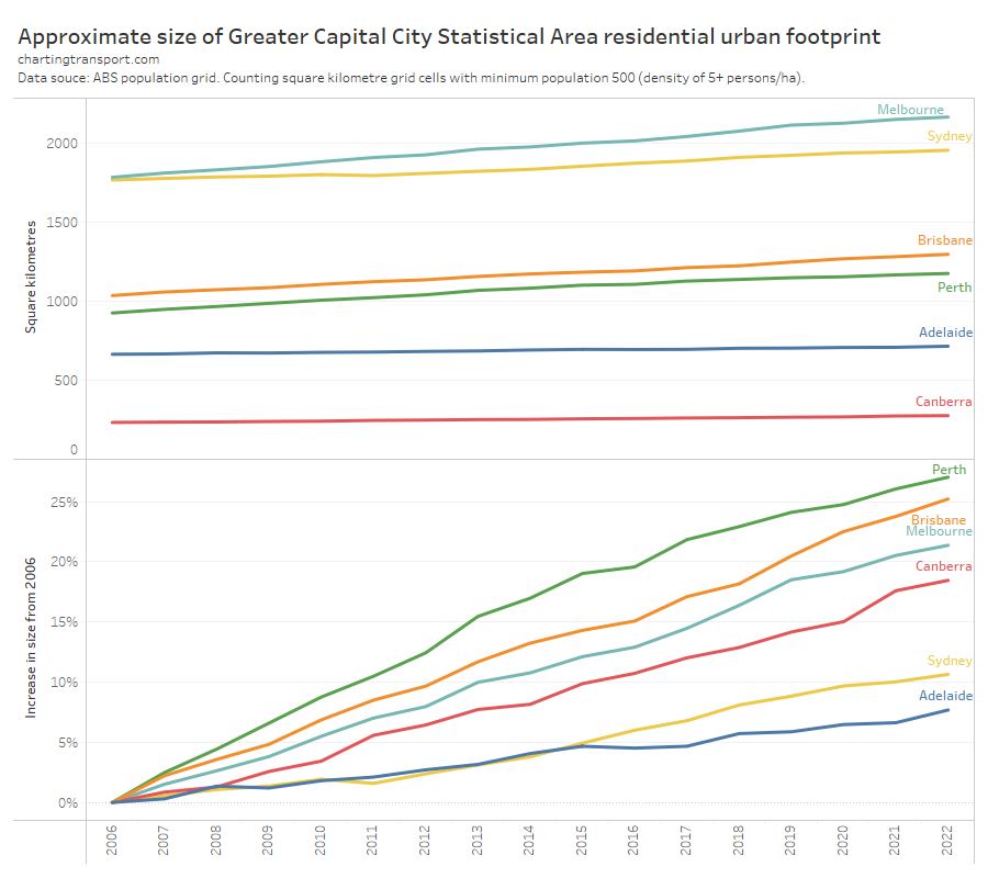
Melbourne and Sydney had much the same footprint in 2006 but Melbourne has since grown significantly larger in size than Sydney, although Sydney still has a larger Capital City Statistical Area population.
The bottom half of the chart shows that Perth has had the largest percentage growth in urban residential area, followed by Brisbane then Melbourne. Sydney and Adelaide have had the least growth in footprint, and are also seeing the least population growth in percentage terms.
Animated density maps of Australian cities
Here are some animated density maps for Australia’s six largest cities from 2006 to 2022 for you to ponder.
Some things to watch for:
- Limited urban sprawl and significant densification of pockets of established areas in Canberra
- Much larger areas of higher density in Sydney and Melbourne
- Relatively high densities in some urban growth areas in Melbourne, Brisbane, and Sydney from the late 2010s
- Low density sprawl in Perth, but also densification of some inner suburban areas (along the Scarborough Beach Road and Wanneroo Road corridors, and inner suburbs like Subiaco and North Perth)
- Limited urban sprawl in Adelaide, along with densification of inner suburbs
Appendix: Corrections to ABS population estimates following Census 2021
The 2021 census resulted in quite large revisions to estimated population in many cities as shown in the following chart.
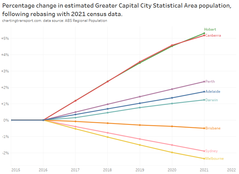
Melbourne’s estimated 2021 population was revised down 2.4%, Sydney down 1.9%, while Canberra and Hobart were revised up more than 5%. To be fair to the ABS, the pandemic and border closures were unprecedented and their impacts on regional population were not easy to predict.
These corrections sum to a linear trend between 2016 and 2021 at the city level, although there was a redistribution of the estimated population within each city.
The following chart shows some detail of estimated population revisions at SA2 level for Melbourne in 2021:
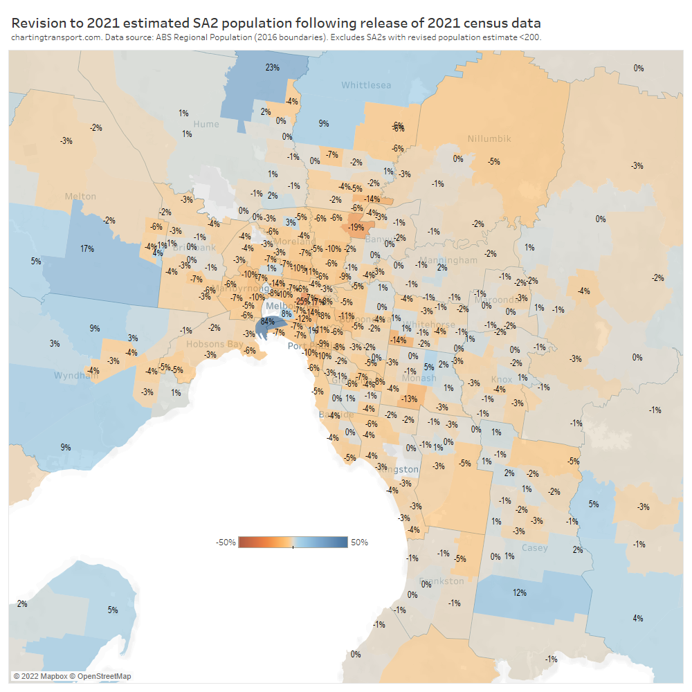
The biggest reduction was in Carlton (-25% right next to University of Melbourne), and there were also reductions near other university campuses, including Kingsbury (-19%), Burwood (-14%) and Clayton (-13%). The biggest upwards revision was Fishermans Bend (+84%), and there were plenty of upwards revisions in outer urban growth areas.
And here is Sydney:
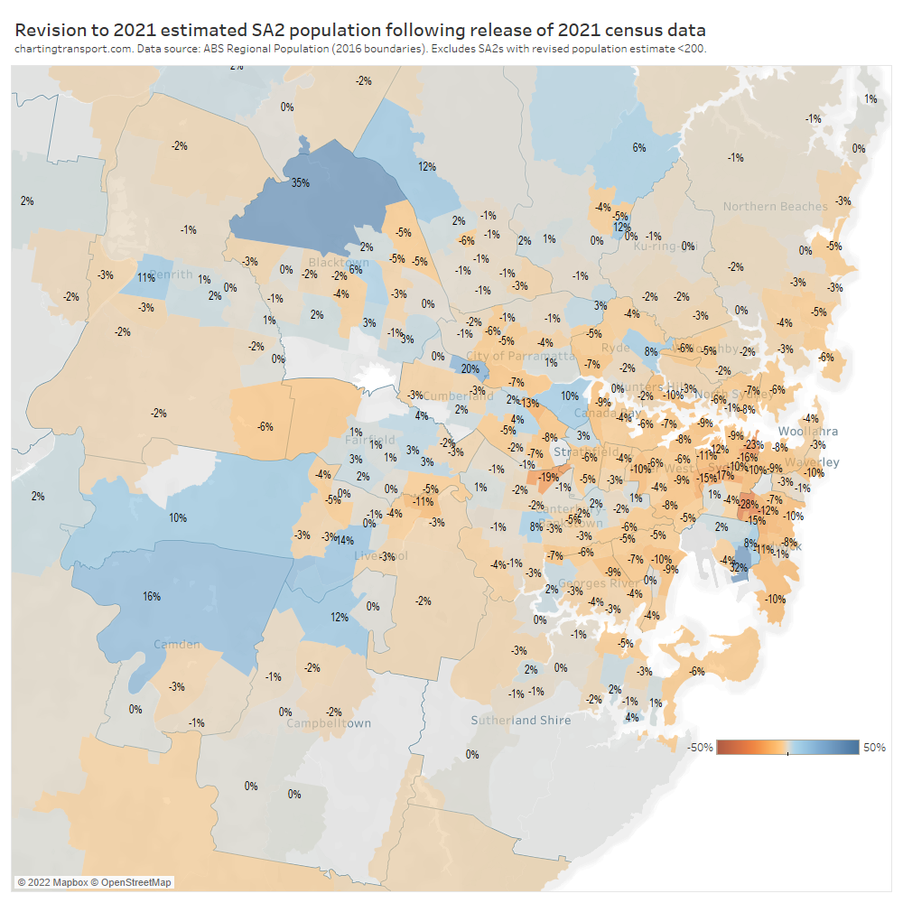
There were big reductions in Kensington (-28%, centred on UNSW), Redfern-Chippendale (-17%), many other areas near university campuses, and around the Sydney CBD.
Like Melbourne, urban growth areas on the fringe were revised upwards, including +35% in Riverstone-Marden Park.


 Posted by chrisloader